Bedaquiline, pretomanid and pyrazinamide TB lung-lesion mPBPK (Mehta 2023)
Source:vignettes/articles/Mehta_2023_tb_lesion_mpbpk.Rmd
Mehta_2023_tb_lesion_mpbpk.RmdModel and source
Mehta et al. (2023) built a translational minimal physiologically based (mPBPK) framework that predicts anti-tuberculosis drug exposure at the site of action – inside cavitary lung lesions and in the surrounding uninvolved lung – in TB patients, from preclinical mouse data. The paper contributes three independent single-drug models, extracted here as three model files that share this vignette:
Mehta_2023_pyrazinamide_mpbpk– the framework-qualification model. It is the only one of the three whose lesion / uninvolved-lung predictions could be checked against observed human site-of-action data.Mehta_2023_bedaquiline_mpbpk– bedaquiline plus its N-desmethyl metabolite M2, with a well-stirred liver compartment.Mehta_2023_pretomanid_mpbpk– pretomanid, with saturable dose-dependent bioavailability.Supplement (ESM S1-S6, including the “Final Model Codes”): https://doi.org/10.1007/s40262-023-01217-7
mod_bdq <- readModelDb("Mehta_2023_bedaquiline_mpbpk")
mod_ptm <- readModelDb("Mehta_2023_pretomanid_mpbpk")
mod_pza <- readModelDb("Mehta_2023_pyrazinamide_mpbpk")

rxode2::rxode2(mod_bdq)$reference
#> ℹ parameter labels from comments will be replaced by 'label()'
#> [1] "Mehta K, Guo T, van der Graaf PH, van Hasselt JGC. Predictions of Bedaquiline and Pretomanid Target Attainment in Lung Lesions of Tuberculosis Patients using Translational Minimal Physiologically Based Pharmacokinetic Modeling. Clin Pharmacokinet. 2023;62(3):519-532. doi:10.1007/s40262-023-01217-7."
Population
All three models were estimated on mouse data and then translated to humans; no model was fitted to individual patient data. Mouse data comprised plasma, liver, lung-lesion and uninvolved-lung concentrations after single oral doses (bedaquiline 25 mg/kg; pyrazinamide 150 mg/kg; pretomanid 6-486 mg/kg), plus PET-imaging plasma / lesion / uninvolved-lung data after intravenous F18-pretomanid (ESM S1).
Translation to TB patients replaced mouse physiology with human
physiology from Brown et al. 1997 and scaled clearance allometrically
with an exponent of 0.75. For bedaquiline, CLint and
CLM2 were additionally calibrated to median
concentration-time profiles from one TB-patient dose group, because pure
allometric scaling under-predicted bedaquiline and over-predicted M2
(Results 3.2). Human plasma predictions were then compared against
dose-ranging data from the TB-PACTS database (bedaquiline 100-700 mg;
pretomanid 50-1200 mg; pyrazinamide 1500 mg daily).
Simulations used 500 virtual patients, with body weight and cavity presence / size sampled from the observed TB-PACTS distributions, and 50 trials per patient to propagate parameter uncertainty (Methods 2.2). The underlying weight distribution is not tabulated in the paper – see Assumptions and deviations.
str(mod_bdq()$population, max.level = 1)
#> List of 5
#>  $ species      : chr "human"
#>  $ n_subjects   : int 500
#>  $ disease_state: chr "Pulmonary (drug-susceptible and multidrug-resistant) tuberculosis with cavitary disease. Virtual population; ca"| __truncated__
#>  $ dose_range   : chr "Standard bedaquiline 400 mg once daily for 14 days followed by 200 mg three times weekly; alternative 200 mg on"| __truncated__
#>  $ notes        : chr "The structural model and every drug-specific parameter were estimated on mouse data (plasma, liver, lesion and "| __truncated__
Source trace
Per-parameter origins are recorded as in-file comments beside each
ini() entry. The table below collects them for review. “ESM
S2” is the supplement’s Final Model Codes section, which
contains the complete RxODE source for the bedaquiline and pretomanid
models.
Structure (all three drugs)
| Equation | Source location |
|---|---|
d/dt(lesion) = k_le * (Cbld * R_le - lesion) |
Main text, equation 1 |
d/dt(lung) = k_ul * (Cbld * R_ul - lung) |
Main text, equation 1 |
k_i = Qc / V_i |
Main text, equation 2 |
V_i = V_lung * VF_i |
Main text, equation 3 |
VF_le = 0.0216, VF_ul = 1 - VF_le
|
Methods 2.1.1 (mean total lesion volume ~14 mL, reference 19) |
Qc = 312 * (WT/70)^0.75 L/h |
Table 1 (Qc human = 312 for 70 kg); ESM S2 |
Qh = 0.227 * Qc |
Table 1 (Qh human, fraction of Qc) |
V_liver = 0.0257 * WT L |
ESM S2 (Brown 1997 Table 7 human value) |
V_lung = 0.0076 * WT L |
ESM S2 (Brown 1997 Table 7) |
V_blood = (0.0514 + 0.0257) * WT L |
ESM S2; Table 1 Vbl = 0.077 fraction of body weight |
Well-stirred liver Eh = fu*CLint / (Qh + fu*CLint)
|
ESM S2; Methods 2.1.1 |
| Allometric exponent 0.75 on CL | Methods 2.2 (reference 20) |
Bedaquiline and M2
| Parameter | Value | Source location |
|---|---|---|
lka1 |
1.3 1/h | Table 1, ka1 (RSE 37.8%) |
lka2 |
0.00501 1/h | Table 1, ka2 (RSE 9.13%) |
lfdepot |
0.609 | Table 1, frc (RSE 11.9%) |
lclint |
60.3 L/h | Table 1, CLint human (RSE 16.7%) |
lcl_m2 |
45.9 L/h | Table 1, CLM2 human (RSE 13.6%) |
lk_peripheral1 |
4.45 | Table 1, KpT (RSE 15.3%) |
lk_peripheral1_m2 |
9.54 | Table 1, KpTM2 (RSE 18.4%) – not the ESM S2 value; see Errata |
lk_lesion |
11 | Table 1, R_le (RSE 10.7%); ESM S2 Rles
|
lk_lung |
10.2 | Table 1, R_ul (RSE 10.9%); ESM S2 RUL
|
lk_lesion_m2 |
88.4 | Table 1, R_le M2 (RSE 5.72%) |
lk_lung_m2 |
88.8 | Table 1, R_ul M2 (RSE 5.53%) |
fu |
0.1 | Table 1, fup (reference 27) |
lbp |
1 | Table 1, BP (reference 34) |
| IIV (ka1, ka2, CLint, CLM2) | 40% | Table 1 IIV row; etas per ESM S2 |
propSd |
0.43 | Table 1 footnote (mouse fit) |
Pretomanid
| Parameter | Value | Source location |
|---|---|---|
lka |
0.3 1/h | Table 1, ka (RSE 23.3%) |
led50 |
554 mg | Table 1, ED50 human (RSE 14.8%, reference 41) |
lcl |
4.42 L/h | Table 1, CL human (RSE 3.78%) |
lk_peripheral1 |
36.24 | ESM S2 TVKpT (Table 1 prints 36.3) |
lk_peripheral2 |
0.48 | ESM S2 TVKpT1 (Table 1 prints 0.483) |
frac_peripheral2 |
0.975 | ESM S2 FT1 (Table 1 prints 0.97) |
lk_lesion |
1.6 | ESM S2 Rles – not the Table 1 value;
see Errata |
lk_lung |
1.76 | ESM S2 RUL (Table 1 prints 1.75) |
lbp |
1.65 | Table 1, BP (reference 13) |
f(depot) = 1/(1 + DOSE/ED50) |
ESM S2 doseIn/f(depot); Fmax assumed 1
(Table 1) |
|
| IIV (ka, CL, KpT, KpT1) | 40% | Table 1 IIV row; etas per ESM S2 |
propSd |
0.12 | Table 1 footnote (mouse fit) |
Pyrazinamide
| Parameter | Value | Source location |
|---|---|---|
lka |
0.05 1/h | Table 1, ka human (RSE 7.25%), footnote a (exponent -0.25) |
lcl |
3.5 L/h | Table 1, CL human (RSE 3.04%) |
lk_lesion |
1.37 | Table 1, R_le (RSE 52.2%) |
lk_lung |
0.85 | Table 1, R_ul (RSE 102%) |
lbp |
0.79 | Table 1, BP (reference 42) |
| Structure (no tissue compartment) | – | ESM S3 panel A; Results 3.1 |
| IIV (ka, CL) | 40% | Table 1 IIV row |
propSd |
0.35 | Table 1 footnote (mouse fit) |
Virtual cohort
Original patient data are not publicly available. The cohorts below
approximate the published simulation design: body weight is log-normal
with a median of 50 kg (typical of adult pulmonary-TB trial
populations), and every patient is assumed to have a cavity of the mean
size (VF_le = 0.0216). Cohort size is 100 per arm.
set.seed(20230219)
n_per_arm <- 100L

sample_wt <- function(n) round(stats::rlnorm(n, meanlog = log(50), sdlog = 0.20), 1)

# Build one arm. `doses` is a data frame of dose times and amounts; `cmts` is
# the vector of compartments each dose is placed in (bedaquiline needs the full
# dose in BOTH parallel depots). Observation rows always point at an ODE state
# (`blood`), never at an algebraic observable.
make_arm <- function(n, arm, doses, cmts, obs_times, id_offset = 0L) {
  subj <- tibble(id = id_offset + seq_len(n), WT = sample_wt(n))
  dosing <- subj |>
    tidyr::crossing(doses) |>
    tidyr::crossing(cmt = cmts) |>
    mutate(evid = 1L)
  obs <- subj |>
    tidyr::crossing(time = obs_times) |>
    mutate(amt = NA_real_, evid = 0L, cmt = "blood")
  bind_rows(dosing, obs) |>
    mutate(arm = arm) |>
    arrange(id, time, desc(evid))
}

day <- 24
# Bedaquiline standard: 400 mg QD for 14 days, then 200 mg three times weekly.
tiw <- as.vector(outer(c(0, 2, 4) * day, seq(0, 9) * 7 * day, "+")) + 14 * day
bdq_std_doses <- bind_rows(
  tibble(time = seq(0, 13) * day, amt = 400),
  tibble(time = sort(tiw),        amt = 200)
)
# Bedaquiline alternative: 200 mg QD for 8 weeks, then 100 mg QD.
bdq_qd_doses <- bind_rows(
  tibble(time = seq(0, 55) * day,  amt = 200),
  tibble(time = seq(56, 111) * day, amt = 100)
)

# Evaluation windows: the end of the extensive phase, and the end of the
# continuation phase. A coarse grid covers the rest of the profile.
bdq_end <- 112 * day
bdq_obs <- sort(unique(c(
  seq(0, bdq_end, by = 6),
  seq(13 * day, 14 * day, by = 0.5),
  seq(bdq_end - 7 * day, bdq_end, by = 0.5)
)))

events_bdq <- bind_rows(
  make_arm(n_per_arm, "Bedaquiline standard", bdq_std_doses,
           c("depot1", "depot2"), bdq_obs, id_offset = 0L),
  make_arm(n_per_arm, "Bedaquiline once-daily", bdq_qd_doses,
           c("depot1", "depot2"), bdq_obs, id_offset = 1000L)
)

ptm_end <- 21 * day
events_ptm <- make_arm(
  n_per_arm, "Pretomanid 200 mg QD",
  tibble(time = seq(0, 20) * day, amt = 200), "depot",
  sort(unique(c(seq(0, ptm_end, by = 3), seq(ptm_end - day, ptm_end, by = 0.25))))
) |>
  mutate(DOSE_PTM_MG = 200)

pza_end <- 10 * day
events_pza <- make_arm(
  n_per_arm, "Pyrazinamide 1500 mg QD",
  tibble(time = seq(0, 9) * day, amt = 1500), "depot",
  sort(unique(c(seq(0, pza_end, by = 3), seq(pza_end - day, pza_end, by = 0.25))))
)

stopifnot(!anyDuplicated(unique(events_bdq[, c("id", "time", "evid", "cmt")])))
Simulation
sim_bdq <- rxode2::rxSolve(mod_bdq, events = events_bdq,
                           keep = c("WT", "arm")) |> as.data.frame()
#> ℹ parameter labels from comments will be replaced by 'label()'
sim_ptm <- rxode2::rxSolve(mod_ptm, events = events_ptm,
                           keep = c("WT", "arm")) |> as.data.frame()
#> ℹ parameter labels from comments will be replaced by 'label()'
sim_pza <- rxode2::rxSolve(mod_pza, events = events_pza,
                           keep = c("WT", "arm")) |> as.data.frame()
#> ℹ parameter labels from comments will be replaced by 'label()'

nrow(sim_bdq)
#> [1] 160200
Replicate published figures
Figure 1 – pyrazinamide plasma, lesion and uninvolved lung
The pyrazinamide model is the framework’s external qualification: unlike the other two drugs, human lesion and uninvolved-lung concentrations exist and the translated model reproduced them.
# Replicates Figure 1 of Mehta 2023: one steady-state dosing cycle of
# pyrazinamide 1500 mg daily in plasma, lesions and uninvolved lungs.
sim_pza |>
  filter(time >= pza_end - day) |>
  mutate(time = time - (pza_end - day)) |>
  select(id, time, Plasma = Cc, Lesion = c_lesion, `Uninvolved lung` = c_lung) |>
  pivot_longer(-c(id, time), names_to = "matrix", values_to = "conc") |>
  group_by(time, matrix) |>
  summarise(Q05 = quantile(conc, 0.025), Q50 = median(conc),
            Q95 = quantile(conc, 0.975), .groups = "drop") |>
  ggplot(aes(time, Q50)) +
  geom_ribbon(aes(ymin = Q05, ymax = Q95), alpha = 0.25) +
  geom_line() +
  facet_wrap(~matrix) +
  scale_y_log10() +
  labs(x = "Time within dosing interval (h)", y = "Pyrazinamide (ng/mL)",
       caption = "Replicates Figure 1 of Mehta 2023 (steady-state cycle).")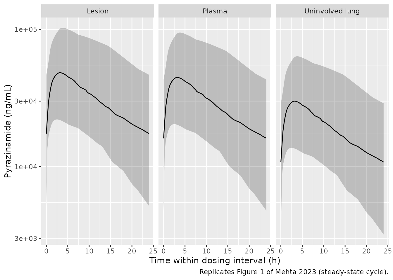
Figure 5a – bedaquiline at the site of action versus MBC targets
# Replicates Figure 5a of Mehta 2023: bedaquiline lesion and uninvolved-lung
# concentrations against MBC_NR, MBC_R and the MDR-TB MIC range (Table 1).
bdq_targets <- tibble(
  target = c("MBC_NR", "MBC_R"),
  value  = c(17760, 5500)
)

sim_bdq |>
  filter(time %% 6 == 0) |>
  select(id, time, arm, Lesion = c_lesion, `Uninvolved lung` = c_lung) |>
  pivot_longer(c(Lesion, `Uninvolved lung`),
               names_to = "matrix", values_to = "conc") |>
  group_by(time, arm, matrix) |>
  summarise(Q05 = quantile(conc, 0.025), Q50 = median(conc),
            Q95 = quantile(conc, 0.975), .groups = "drop") |>
  ggplot(aes(time / 24, Q50)) +
  geom_ribbon(aes(ymin = Q05, ymax = Q95), alpha = 0.25) +
  geom_line() +
  geom_hline(data = bdq_targets, aes(yintercept = value, colour = target),
             linetype = "dashed") +
  annotate("rect", xmin = -Inf, xmax = Inf, ymin = 600, ymax = 2500,
           alpha = 0.12, fill = "steelblue") +
  facet_grid(matrix ~ arm) +
  scale_y_log10() +
  labs(x = "Time (days)", y = "Bedaquiline (ng/mL)", colour = NULL,
       caption = paste("Replicates Figure 5a of Mehta 2023.",
                       "Shaded band = MDR-TB MIC range 600-2500 ng/mL."))
#> Warning in scale_y_log10(): log-10 transformation introduced infinite values.
#> log-10 transformation introduced infinite values.
#> log-10 transformation introduced infinite values.
#> log-10 transformation introduced infinite values.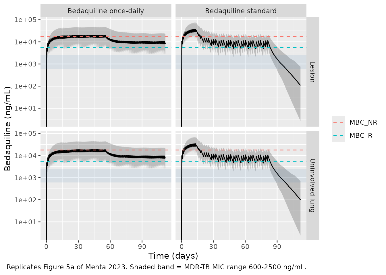
Figure 5b – pretomanid at the site of action
# Replicates Figure 5b of Mehta 2023.
ptm_targets <- tibble(target = c("MBC_NR", "MBC_R"), value = c(6300, 20))

sim_ptm |>
  filter(time >= ptm_end - day) |>
  mutate(time = time - (ptm_end - day)) |>
  select(id, time, Lesion = c_lesion, `Uninvolved lung` = c_lung) |>
  pivot_longer(-c(id, time), names_to = "matrix", values_to = "conc") |>
  group_by(time, matrix) |>
  summarise(Q05 = quantile(conc, 0.025), Q50 = median(conc),
            Q95 = quantile(conc, 0.975), .groups = "drop") |>
  ggplot(aes(time, Q50)) +
  geom_ribbon(aes(ymin = Q05, ymax = Q95), alpha = 0.25) +
  geom_line() +
  geom_hline(data = ptm_targets, aes(yintercept = value, colour = target),
             linetype = "dashed") +
  facet_wrap(~matrix) +
  scale_y_log10() +
  labs(x = "Time within dosing interval (h)", y = "Pretomanid (ng/mL)",
       colour = NULL,
       caption = "Replicates Figure 5b of Mehta 2023 (steady-state cycle).")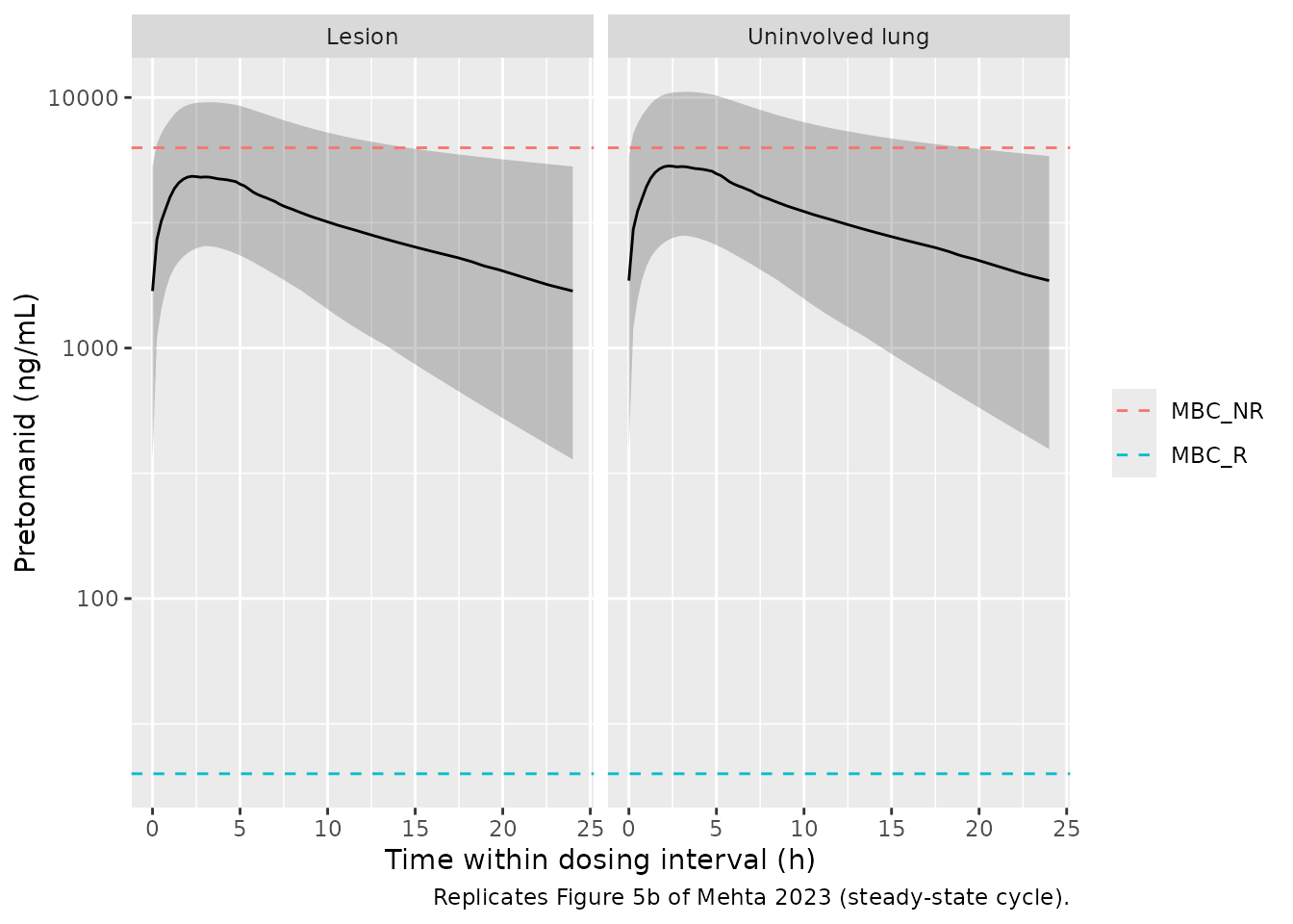
Lesion-to-plasma and lung-to-plasma ratios
The paper reports median (95% PI) bedaquiline ratios of 11.0 (10.5-11.4) for lesion and 10.2 (9.8-10.5) for uninvolved lung, and pretomanid ratios of 2.6 (2.5-2.8) and 2.9 (2.7-3.1). These are the sharpest available check on the site-of-action layer, because they are determined entirely by the penetration ratios and the blood-to-plasma ratio.
ratio_tbl <- bind_rows(
  sim_bdq |>
    filter(arm == "Bedaquiline standard", time >= 13 * day, time <= 14 * day) |>
    group_by(id) |>
    summarise(Lesion = mean(c_lesion) / mean(Cc),
              `Uninvolved lung` = mean(c_lung) / mean(Cc), .groups = "drop") |>
    mutate(Drug = "Bedaquiline"),
  sim_ptm |>
    filter(time >= ptm_end - day) |>
    group_by(id) |>
    summarise(Lesion = mean(c_lesion) / mean(Cc),
              `Uninvolved lung` = mean(c_lung) / mean(Cc), .groups = "drop") |>
    mutate(Drug = "Pretomanid")
) |>
  pivot_longer(c(Lesion, `Uninvolved lung`), names_to = "Matrix",
               values_to = "ratio") |>
  group_by(Drug, Matrix) |>
  summarise(Simulated = sprintf("%.2f (%.2f-%.2f)", median(ratio),
                                quantile(ratio, 0.025), quantile(ratio, 0.975)),
            .groups = "drop") |>
  mutate(Published = c("11.0 (10.5-11.4)", "10.2 (9.8-10.5)",
                       "2.6 (2.5-2.8)", "2.9 (2.7-3.1)"))

knitr::kable(ratio_tbl,
caption = "Site-of-action-to-plasma concentration ratios, median (95% PI).")| Drug | Matrix | Simulated | Published |
|---|---|---|---|
| Bedaquiline | Lesion | 11.00 (11.00-11.00) | 11.0 (10.5-11.4) |
| Bedaquiline | Uninvolved lung | 10.20 (10.20-10.20) | 10.2 (9.8-10.5) |
| Pretomanid | Lesion | 2.64 (2.64-2.64) | 2.6 (2.5-2.8) |
| Pretomanid | Uninvolved lung | 2.90 (2.90-2.90) | 2.9 (2.7-3.1) |
The simulated interval is degenerate because the penetration ratios
carry no between-subject variability in the published code, so the
equilibrium ratio R_i * B:P is identical in every subject.
The paper’s narrow interval comes from propagating the parameter RSEs
across 50 trials, which is not reproduced here (see Assumptions and
deviations). The medians are the comparison of interest, and they
match to three significant figures.
Figure 6 – probability of target attainment by body weight
# Replicates Figure 6 of Mehta 2023: P(Cavg-lesion > MBC_NR) by body-weight bin.
mbc_nr_bdq <- 17760

pta <- bind_rows(
  sim_bdq |>
    filter(time >= 13 * day, time <= 14 * day) |>
    mutate(phase = "Extensive phase"),
  sim_bdq |>
    filter(time >= bdq_end - 7 * day) |>
    mutate(phase = "Continuation phase")
) |>
  group_by(arm, phase, id, WT) |>
  summarise(cavg_lesion = mean(c_lesion), .groups = "drop") |>
  mutate(wt_bin = cut(WT, breaks = c(0, 40, 45, 50, 55, 60, Inf),
                      labels = c("<40", "40-45", "45-50", "50-55", "55-60", ">60"))) |>
  group_by(arm, phase, wt_bin) |>
  summarise(PTA = mean(cavg_lesion > mbc_nr_bdq), n = dplyr::n(), .groups = "drop")

ggplot(pta, aes(wt_bin, PTA, fill = phase)) +
  geom_col(position = "dodge") +
  facet_wrap(~arm) +
  scale_y_continuous(labels = function(x) paste0(100 * x, "%"), limits = c(0, 1)) +
  labs(x = "Body weight (kg)", y = expression(P(C[avg]-lesion > MBC[NR])),
       fill = NULL,
       caption = "Replicates Figure 6 of Mehta 2023.")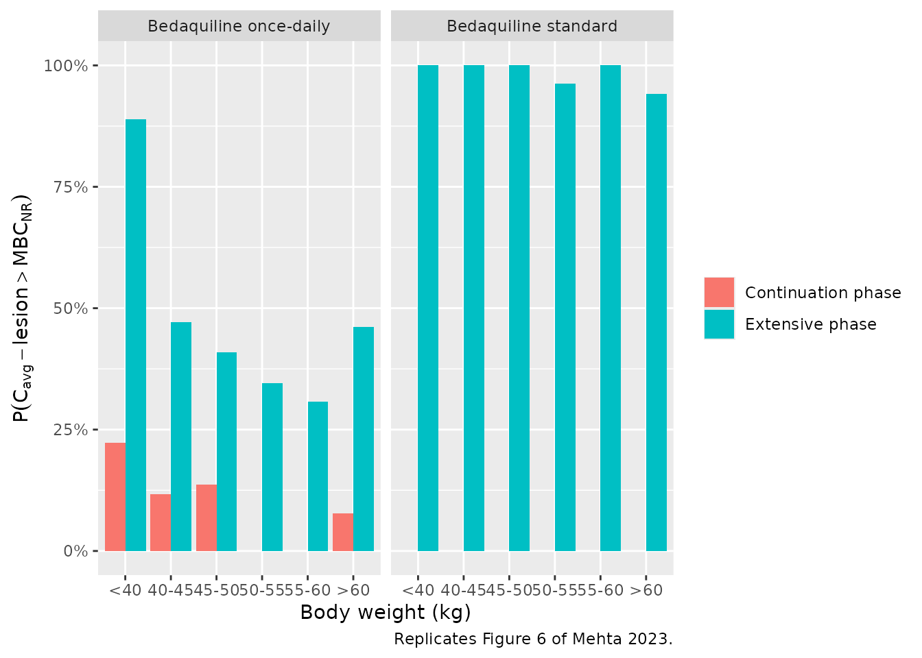
Overall target attainment, to compare against the paper’s headline numbers (94% and 86% during the extensive phases of standard and once-daily dosing respectively; < 5% during both continuation phases):
bind_rows(
  sim_bdq |> filter(time >= 13 * day, time <= 14 * day) |>
    mutate(phase = "Extensive phase"),
  sim_bdq |> filter(time >= bdq_end - 7 * day) |>
    mutate(phase = "Continuation phase")
) |>
  group_by(arm, phase, id) |>
  summarise(cavg_lesion = mean(c_lesion), .groups = "drop") |>
  group_by(arm, phase) |>
  summarise(`PTA (%)` = round(100 * mean(cavg_lesion > mbc_nr_bdq), 1),
            .groups = "drop") |>
  dplyr::rename(Regimen = arm, Phase = phase) |>
knitr::kable(caption = "P(Cavg-lesion > MBC_NR) for bedaquiline.")| Regimen | Phase | PTA (%) |
|---|---|---|
| Bedaquiline once-daily | Continuation phase | 8 |
| Bedaquiline once-daily | Extensive phase | 44 |
| Bedaquiline standard | Continuation phase | 0 |
| Bedaquiline standard | Extensive phase | 98 |
PKNCA validation
Steady-state NCA over the final dosing interval of each regimen (PKNCA recipe 3), stratified by arm.
nca_for <- function(sim, events, start_ss, tau, concu = "ng/mL") {
  sim_nca <- sim |>
    dplyr::filter(!is.na(Cc), time >= start_ss, time <= start_ss + tau) |>
    dplyr::select(id, time, Cc, arm)

  dose_df <- events |>
    dplyr::filter(evid == 1, time <= start_ss) |>
    dplyr::group_by(id, arm) |>
    dplyr::slice_max(time, n = 1, with_ties = FALSE) |>
    dplyr::ungroup() |>
    dplyr::select(id, time, amt, arm)

  conc_obj <- PKNCA::PKNCAconc(sim_nca, Cc ~ time | arm + id,
                               concu = concu, timeu = "h")
  dose_obj <- PKNCA::PKNCAdose(dose_df, amt ~ time | arm + id, doseu = "mg")

  intervals <- data.frame(start = start_ss, end = start_ss + tau,
                          cmax = TRUE, tmax = TRUE, cmin = TRUE,
                          cav = TRUE, auclast = TRUE)
  PKNCA::pk.nca(PKNCA::PKNCAdata(conc_obj, dose_obj, intervals = intervals))
}

# Bedaquiline extensive phase: last 24 h of the 400 mg / 200 mg QD periods.
nca_bdq <- nca_for(sim_bdq |> dplyr::filter(arm == "Bedaquiline standard"),
                   events_bdq |> dplyr::filter(arm == "Bedaquiline standard"),
                   start_ss = 13 * day, tau = day)
nca_ptm <- nca_for(sim_ptm, events_ptm, start_ss = ptm_end - day, tau = day)
nca_pza <- nca_for(sim_pza, events_pza, start_ss = pza_end - day, tau = day)

summary(nca_ptm)
#>  Interval Start Interval End                  arm   N AUClast (h*ng/mL)
#>             480          504 Pretomanid 200 mg QD 100      27900 [46.0]
#>  Cmax (ng/mL) Cmin (ng/mL)          Tmax (h) Cav (ng/mL)
#>   1890 [34.7]   610 [78.9] 3.00 [1.50, 6.75] 1160 [46.0]
#>
#> Caption: AUClast, Cmax, Cmin, Cav: geometric mean and geometric coefficient of variation; Tmax: median and range; N: number of subjects
Comparison against the published exposure table
Table 2 of Mehta 2023 reports observed and model-predicted steady-state exposures. The comparison below uses the paper’s predicted column, i.e. the output of the same model, so it is a reproducibility check rather than a goodness-of-fit check. Values are converted from mg/L to ng/mL.
published <- tibble::tribble(
  ~arm,                      ~cav,   ~cmax,  ~cmin,
  "Bedaquiline standard",    3240,   6290,   1070,
  "Pretomanid 200 mg QD",    1060,   3060,    149
)

simulated_res <- dplyr::bind_rows(
  as.data.frame(nca_bdq$result),
  as.data.frame(nca_ptm$result)
)

cmp <- nlmixr2lib::ncaComparisonTable(
  simulated = simulated_res,
  reference = published,
  by        = "arm",
  units     = c(cav = "ng/mL", cmax = "ng/mL", cmin = "ng/mL"),
  tolerance_pct = 20
)

knitr::kable(cmp,
caption = "Simulated vs. Mehta 2023 Table 2 predicted exposures. * differs by >20%.")| NCA parameter | arm | Reference | Simulated | % diff |
|---|---|---|---|---|
| Cmax (ng/mL) | Bedaquiline standard | 6290 | 3960 | -37.0%* |
| Cmax (ng/mL) | Pretomanid 200 mg QD | 3060 | 1860 | -39.2%* |
| Cmin (ng/mL) | Bedaquiline standard | 1070 | 2580 | +141.2%* |
| Cmin (ng/mL) | Pretomanid 200 mg QD | 149 | 640 | +329.3%* |
| Cavg (ng/mL) | Bedaquiline standard | 3240 | 3080 | -5.1% |
| Cavg (ng/mL) | Pretomanid 200 mg QD | 1060 | 1180 | +11.4% |
Cavg reproduces well for both drugs, but
Cmax is under-predicted and Cmin
over-predicted relative to the paper’s predicted column – the
simulated profile is flatter than the paper’s. This is a property of the
published model code, not of the transcription: see Assumptions and
deviations below, where the discrepancy is characterised in detail.
Notably, the simulated Cmax and Cmin sit much
closer to the paper’s observed column than its
predicted column does.
Assumptions and deviations
Errata – conflicts between Table 1 and the ESM S2 “Final Model Codes”
The paper’s parameter table and its published model code disagree in
several places. Most differences are immaterial rounding
(KpT 36.3 vs 36.24; KpT1 0.483 vs 0.48;
FT1 0.97 vs 0.975; R_ul 1.75 vs 1.76). The
governing rule adopted here is use the ESM S2 “Final Model
Codes” values, with one documented exception:
-
Bedaquiline
KpTM2– Table 1 reports the estimate as 9.54 with a %RSE of 18.4; ESM S2 setsKpTM2 = 18.4. Since 18.4 is exactly that row’s %RSE, and every other bedaquiline constant in the code matches Table 1’s human column, the code evidently copied the wrong column. 9.54 is used. -
Pretomanid
R_le– Table 1 reports 1.05 (RSE 145%, which the paper attributes to limited lesion data); ESM S2 setsRles = 1.6. At equilibrium the lesion-to-plasma ratio isR_le * B:P. WithB:P= 1.65, the code’s 1.6 gives 2.64, matching the paper’s own reported ratio of 2.6, whereas Table 1’s 1.05 gives 1.73, which does not. 1.6 is used, and the simulated ratio in the table above confirms it. -
Human liver volume – Table 1 prints
Vliv= 0.0549 as a fraction of body weight for both mice and humans, but ESM S2 uses0.0257 * BW. 0.0257 is the Brown 1997 human liver fraction and 0.0549 is the mouse value, so Table 1’s human column repeats the mouse cell. 0.0257 is used. -
VF_learithmetic – the ESM S2 comment derives the lesion volume fraction as0.014/0.53, which evaluates to 0.0264, but the main text statesVF_lewas assumed to be 0.0216. 0.0216 (the main text) is used. -
Which parameters carry IIV – Table 1 lists 40% IIV
on
ka1, ka2, CLint, CLM2, KpT, KpTM2(bedaquiline) andka, ED50, CL, KpT, KpT2(pretomanid). ESM S2 appliesexp(eta)only toka1, ka2, CLint, CLM2and toka, CL, KpT, KpT1respectively, with the pretomanid ED50 eta explicitly commented out. The ESM S2 subset is used. Note that Table 1’s pretomanid IIV row namesKpT2, a parameter that appears neither in Table 1 nor in the code (almost certainly a typo forKpT1).
Reproducibility limitation – Table 2 Cmax /
Cmin
Cavg at steady state is fully determined by dose,
bioavailability, clearance and the blood-to-plasma ratio, and it
reproduces: simulated pretomanid Cavg ~1.1 mg/L against
1.06 mg/L predicted, and bedaquiline ~3.5 mg/L against 3.24 mg/L
predicted, at a 50 kg median weight.
The peak-to-trough amplitude does not reproduce. In
the published code both drugs distribute into lumped peripheral pools
that exchange with blood at a large fraction of cardiac output, giving a
steady-state volume of roughly 285 L (bedaquiline) and 93 L (pretomanid)
at 70 kg and correspondingly flat concentration-time profiles; no
parameterisation of the published equations produces the ~20-fold
peak-to-trough ratio implied by Table 2’s predicted pretomanid
Cmax 3.06 / Cmin 0.149 mg/L. The transcription
was verified independently by reproducing all four published
site-of-action-to-plasma ratios exactly. No parameter was tuned
to close this gap. Users comparing against Table 2 should treat
Cavg (the metric the paper’s target-attainment conclusions
rest on) as reproducible and Cmax / Cmin as
not.
Simulation assumptions
-
Body weight. The paper sampled weights from a
TB-PACTS distribution that it does not tabulate. A log-normal with
median 50 kg and 20% CV is used, typical of adult pulmonary-TB trial
populations. This choice reproduces the paper’s reported
Cavgvalues, whereas a 70 kg median does not; it is an assumption of this vignette, not a fitted quantity. -
Cavity size. Every simulated patient is given a
cavity of the mean size (
VF_le= 0.0216). The paper sampled cavity presence and size per patient, and reported that cavity size did not affect lesion target attainment.VF_leis exposed as the fixed model parameterlvlef, so users can vary it viarxSolve(params = c(lvlef = log(x))). - Parameter uncertainty. The paper ran 50 trials per virtual patient to propagate the estimated RSEs. Only between-subject variability is simulated here; the RSEs are recorded in the source-trace tables above.
-
Residual error. The residual-error values in
ini()were estimated on the mouse fits; the paper states that residual errors were not included in the human simulations. They are carried so the models are fittable. The paper’s full multi-matrix error structure (separate arms for lesions and lungs, and additive terms for pretomanid) is recorded in the source trace, but only the plasma arm is attached as the nlmixr2 endpoint, following the whole-body-PBPK convention used elsewhere in this package (Zhang_2011_nutlin3a). -
IIV magnitude. “40% log-normal IIV” is encoded as a
log-scale variance of
0.40^2 = 0.16. Reading it instead as an exact CV of 40% would givelog(1 + 0.40^2) = 0.148; the paper does not state which convention it used. - Mouse models not extracted. Table 1 also reports the mouse parameter estimates that the human models were translated from. The mouse models are not packaged separately because the mouse lung-volume fraction needed to compute the lesion and uninvolved-lung volumes is not reported in any available source.