Apricoxib / CS-706 (Kastrissios 2006)
Source:vignettes/articles/Kastrissios_2006_apricoxib.Rmd
Kastrissios_2006_apricoxib.RmdModel and source
#> ℹ parameter labels from comments will be replaced by 'label()'Citation: Kastrissios H, Rohatagi S, Moberly J, Truitt K, Gao Y, Wada R, Takahashi M, Kawabata K, Salazar D. (2006). Development of a Predictive Pharmacokinetic Model for a Novel Cyclooxygenase-2 Inhibitor. Journal of Clinical Pharmacology 46(5):537-548. doi:10.1177/0091270006287122. The paper names the compound only by its Sankyo development code CS-706; the INN subsequently assigned to that molecule (2-(4-ethoxyphenyl)-4-methyl-1-(4-sulfamoylphenyl)-pyrrole, CAS 197904-84-0) is apricoxib, which this file uses per the library’s generic-name-over-development-code convention.
Description: Two-compartment population PK model with first-order absorption and an absorption lag time for the selective cyclooxygenase-2 (COX-2) inhibitor apricoxib (development code CS-706) in 104 healthy adult volunteers across three phase 1 studies (2 to 800 mg single or twice-daily doses for up to 14 days). The model carries three nonlinearities the authors identified and retained. (1) Relative bioavailability saturates with dose according to a standard saturation (Emax) model, Frel = D50 / (Dose + D50) with D50 = 221 mg, so Frel halves at 221 mg. (2) The same Frel is increased exp(0.351) = 1.42-fold for an evening dose relative to a morning dose, reproducing the apparent diurnal variation in exposure seen on both day 1 and day 14 of the twice-daily study. (3) Apparent oral clearance takes a separate typical value at the two supratherapeutic dose levels (400 and 800 mg, DOSE_HIGH = 1), 19.5 L/h versus 34.1 L/h. Covariate effects on CL/F are sex (SEXF), the pooled poor-or-intermediate CYP2D6 phenotype (CYP2D6_PM_IM) and the CYP2C9 reduced-hydroxylator phenotype (CYP2C9_RH); central volume scales as a power of body weight normalised to the 73.3 kg cohort median. Exponential IIV on all six disposition and absorption parameters, proportional residual error. Absolute bioavailability F was not identifiable and was set to 1 by the authors, so all clearance and volume terms are apparent (CL/F, Vc/F, Vp/F, Q/F).
The paper names the compound only by its Sankyo development code CS-706. The INN later assigned to that molecule (2-(4-ethoxyphenyl)-4-methyl-1-(4-sulfamoylphenyl)-pyrrole, CAS 197904-84-0) is apricoxib, which this model file uses per the library’s generic-name-over-development-code convention. The identity is corroborated inside the paper itself: its bioanalytical section reports CS-706 detected at m/z 357, matching apricoxib’s protonated molecular ion (MW 356.4).
No supplement is referenced by the article, and no erratum exists
(the PubMed record for PMID 16638737 carries no Erratum in
notice).
Population
The model was developed from 104 apricoxib-treated healthy adult volunteers across three phase 1 studies conducted at a single United States site (Kastrissios 2006 Table II, development-data-set column):
- Study 1 – single doses of 2, 5, 10, 25, 50, 100 or 200 mg (n = 56), serial sampling to 72 h.
- Study 2 – single doses of 400 or 800 mg (n = 16), serial sampling to 72 h (400 mg) or 144 h (800 mg).
- Study 3 – 25, 100 or 200 mg twice daily for 14 days (n = 32), 12-h profiles after the first two and final two doses plus troughs on days 2-13 and to 72 h after the last dose.
Sex was exactly balanced (52 male / 52 female), median age 27.0 y (19-46), median weight 73.3 kg (49.5-104), median height 173 cm (150-191), median BMI 25.3 kg/m^2 (19.3-29.3), and the cohort was 88.5% white. All doses were given under fasted conditions. Estimation was FOCE in NONMEM v5 (Table III run 19, objective function 15000).
The abstract’s “130 subjects” counts everyone randomised,
including placebo: subjects were allocated to active or placebo at a 4:1
ratio (8 active and 2 placebo per dose level, 70 + 20 + 40 = 130), and
“placebo and missing CS-706 plasma concentration data were excluded from
the NONMEM data sets”. The 104 figure is therefore the number of
subjects that actually informed the fit, and is what this model’s
population metadata records.
A separate 80-subject phase 1 upper-gastrointestinal endoscopic-surveillance study supplied the external validation data set: a single trough concentration 24 h after the seventh daily 100 mg or 200 mg dose. Its subjects are not part of the 104, and its CYP phenotypes were not collected, so the paper’s validation simulation drew phenotype distributions from the development set.
str(ui$population, max.level = 1)
#> List of 13
#>  $ species       : chr "human"
#>  $ n_subjects    : int 104
#>  $ n_studies     : int 3
#>  $ age_range     : chr "19-46 years"
#>  $ age_median    : chr "27.0 years"
#>  $ weight_range  : chr "49.5-104 kg"
#>  $ weight_median : chr "73.3 kg"
#>  $ sex_female_pct: num 50
#>  $ race_ethnicity: Named num [1:5] 88.5 2.9 1.9 3.8 2.9
#>   ..- attr(*, "names")= chr [1:5] "White" "Black" "Asian" "Hispanic" ...
#>  $ disease_state : chr "healthy adult volunteers"
#>  $ dose_range    : chr "Oral apricoxib (CS-706). Study 1: single doses of 2, 5, 10, 25, 50, 100 or 200 mg (n = 56 active), serial sampl"| __truncated__
#>  $ regions       : chr "United States (single phase 1 site: MDS Pharma Services, Lincoln, Nebraska)"
#>  $ notes         : chr "Baseline characteristics from Table II, development data set column. n_subjects = 104 counts only apricoxib-tre"| __truncated__
Source trace
Every ini() entry in
inst/modeldb/specificDrugs/Kastrissios_2006_apricoxib.R
carries an in-file comment naming its source location. They are
collected here for review. None of the eight equations survives naive
plain-text extraction of the PDF; the equation forms below were
recovered verbatim with pdftotext -layout.
| Equation / parameter | Value | Source location |
|---|---|---|
Exponential IIV, theta_i = theta_T * exp(eta_i)
|
n/a | Equation 1, p. 539 |
Proportional residual error, y = yhat * (1 + eps)
|
n/a | Equation 3 (final model), p. 539 |
Continuous covariate, theta_T * (Cov/Cov_med)^Kcov
|
n/a | Equation 4, p. 539 |
Categorical covariate, theta_T * exp(Cov * Kcov)
|
n/a | Equation 5, p. 539 |
frel = 1 * exp(K_Frel-PM * PM) * D50/(DOSE + D50) |
n/a | Equation 6, p. 542 |
CL/F = [CL_Typ*(1-Dhi) + CL_Typ,hi*Dhi] * exp(Sex*K_SEX) * exp(CYPD*K_2D6) * exp(CYPC*K_2C9) |
n/a | Equation 7, p. 542 |
Vc/F = Vc_Typ * (Weight/73.3)^K_Vc-WT |
n/a | Equation 8, p. 542 |
| Two-compartment disposition, first-order absorption + lag | n/a | Results p. 541-542; Table III runs 2 and 4; Discussion p. 545 |
lvc (Vc/F) |
166 L | Table IV |
lvp (Vp/F) |
483 L | Table IV |
lq (Q/F) |
75 L/h | Table IV |
lcl (CL/F, 2-200 mg) |
34.1 L/h | Table IV |
lcl_highdose (CL/F, 400-800 mg) |
19.5 L/h | Table IV |
lka (KA) |
0.542 1/h | Table IV |
ltlag (TLAG) |
0.236 h | Table IV |
led50 (D50 for F) |
221 mg | Table IV |
e_evening_fdepot (K_Frel-PM) |
0.351 | Table IV |
e_sexf_cl (K_CL/F-SEX) |
0.325 | Table IV |
e_cyp2d6_pmim_cl (K_CL/F-CYP2D6) |
-1.01 | Table IV |
e_cyp2c9_rh_cl (K_CL/F-CYP2C9) |
-0.163 | Table IV (printed “-00.163”; see Errata) |
e_wt_vc (K_Vc/F-WT) |
0.831 | Table IV |
etalvc, etalvp, etalq,
etalcl, etalka, etaltlag
|
0.127, 0.234, 0.229, 0.125, 0.052, 0.002 | Table IV, omega^2 rows |
propSd |
sqrt(0.069) = 0.2627 |
Table IV, sigma^2 row |
| Indicator definitions (Dhi, Sex, CYPD, CYPC, PM) | n/a | Paragraph following equation 8, p. 542 |
| Simulation demographics (Japanese vs Western) | n/a | Table I |
Table IV reports omega^2 and sigma^2 as
variances: its “Estimated Variability (%)” column is
footnote b’s sqrt(omega^2), which reproduces every printed
row.
The tolerance for this check is set by the paper’s own printed
precision, not chosen by hand. Table IV prints each variance to three
decimals, so a printed omega^2 of x means the
true value lies in [x - 0.0005, x + 0.0005] and the implied
CV lies in 100 * sqrt() of that interval. The published CV
must fall inside it. This matters: sqrt(0.002) is 4.47%
while Table IV prints 4.36% for omega^2 Tlag, which looks
like a mismatch until the rounding is propagated – 4.36% corresponds to
an unrounded variance of 0.0019, comfortably inside the interval that
rounds to 0.002. A flat tolerance would either miss that or fail
spuriously.
tab4 <- tibble::tribble(
  ~parameter, ~omega2, ~printed_cv,
  "Vc/F",     0.127,   35.6,
  "Vp/F",     0.234,   48.4,
  "Q/F",      0.229,   47.9,
  "CL/F",     0.125,   35.4,
  "Ka",       0.052,   22.7,
  "Tlag",     0.002,   4.36,
  "sigma^2",  0.069,   26.3
) |>
  dplyr::mutate(
    cv_low  = 100 * sqrt(pmax(0, omega2 - 0.0005)),
    cv_high = 100 * sqrt(omega2 + 0.0005),
    consistent = printed_cv >= cv_low & printed_cv <= cv_high
  )

# Enumerating gate: every row of the variability column, not a sample.
stopifnot(nrow(tab4) == 7L, all(tab4$consistent))

tab4 |>
  dplyr::mutate(dplyr::across(c(cv_low, cv_high), \(x) round(x, 2))) |>
  dplyr::rename("Parameter" = parameter, "Variance (Table IV)" = omega2,
                "Published variability (%)" = printed_cv,
                "Implied CV%, low" = cv_low, "Implied CV%, high" = cv_high,
                "Consistent" = consistent) |>
  knitr::kable(caption = paste(
    "Table IV's variance rows reproduce its published variability column once",
"the three-decimal rounding of each variance is propagated."))| Parameter | Variance (Table IV) | Published variability (%) | Implied CV%, low | Implied CV%, high | Consistent |
|---|---|---|---|---|---|
| Vc/F | 0.127 | 35.60 | 35.57 | 35.71 | TRUE |
| Vp/F | 0.234 | 48.40 | 48.32 | 48.43 | TRUE |
| Q/F | 0.229 | 47.90 | 47.80 | 47.91 | TRUE |
| CL/F | 0.125 | 35.40 | 35.28 | 35.43 | TRUE |
| Ka | 0.052 | 22.70 | 22.69 | 22.91 | TRUE |
| Tlag | 0.002 | 4.36 | 3.87 | 5.00 | TRUE |
| sigma^2 | 0.069 | 26.30 | 26.17 | 26.36 | TRUE |
Structural gates: every numeric claim in the abstract and Discussion
The paper reports no NCA table – AUC0-24 appears
only as the axis of Figures 6 and 7 (mean +- SD plots whose values are
not printed), and Cmax / Tmax are discussed only qualitatively. What it
does report is a set of model-derived numeric claims, and each
one is a sharp deterministic gate on the packaged model. Every gate
below is typical-value (zeroRe()), so no seed or cohort is
involved.
mod <- readModelDb("Kastrissios_2006_apricoxib")
modt <- mod |> rxode2::zeroRe()
#> ℹ parameter labels from comments will be replaced by 'label()'

# `rxSolve` on an rxUi scales QUADRATICALLY in the number of subjects passed in
# a SINGLE call. Measured on rxode2 5.1.7 with this model and event grid:
# 45 subjects 0.5 s, 90 -> 1.5 s, 180 -> 7 s, 360 -> 37 s, 900 -> 394 s. (The
# same events through a plain `rxode2::rxode2({})` copy of the model take
# 0.2 s at 180 subjects, so the cost is in the rxUi solve path, not the ODEs,
# and it is unrelated to `keep =`, to the etas, or to `returnType`.)
#
# Splitting one big call into one call per arm keeps the cohort size the
# vignette wants while making the solve linear in the number of arms: the
# Figure 1 simulation below drops from ~6.5 minutes to ~15 seconds. Subject IDs
# are disjoint across arms, so the results are identical to a single call apart
# from which eta draws land on which subject.
solve_by_arm <- function(m, ev, arm_col, keep = character()) {
  stopifnot(arm_col %in% names(ev), arm_col %in% keep)
  parts <- split(ev, ev[[arm_col]])
  stopifnot(length(parts) >= 1L)
  dplyr::bind_rows(lapply(parts, function(p) {
    as.data.frame(rxode2::rxSolve(m, p, keep = keep))
  }))
}
# Solve one 24-h profile per covariate stratum and read the model's own
# derived `cl`, `vc` and `frel` back out.
strata <- tidyr::expand_grid(
  SEXF = c(0, 1), CYP2D6_PM_IM = c(0, 1), CYP2C9_RH = c(0, 1),
  DOSE_HIGH = 0, WT = 73.3, dose = 200
) |>
  dplyr::mutate(id = dplyr::row_number())

ev_strata <- dplyr::bind_rows(
  strata |> dplyr::mutate(time = 0, amt = dose, evid = 1L, cmt = "depot"),
  strata |> tidyr::expand_grid(t_obs = c(2, 12)) |>
    dplyr::mutate(time = t_obs, amt = NA_real_, evid = 0L, cmt = "central") |>
    dplyr::select(-t_obs)
) |>
  dplyr::arrange(id, time, dplyr::desc(evid)) |>
  as.data.frame()

s_strata <- rxode2::rxSolve(modt, ev_strata,
                            keep = c("SEXF", "CYP2D6_PM_IM", "CYP2C9_RH")) |>
  as.data.frame() |>
  dplyr::filter(!is.na(Cc)) |>
  dplyr::group_by(id, SEXF, CYP2D6_PM_IM, CYP2C9_RH) |>
  dplyr::summarise(cl = dplyr::first(cl), vc = dplyr::first(vc), .groups = "drop")
#> ℹ omega/sigma items treated as zero: 'etalvc', 'etalvp', 'etalq', 'etalcl', 'etalka', 'etaltlag'
#> Warning: multi-subject simulation without without 'omega'

# Closed form of equation 7 at DOSE_HIGH = 0, WT = 73.3.
s_strata <- s_strata |>
  dplyr::mutate(cl_closed = 34.1 * exp(0.325 * (1 - SEXF)) *
                  exp(-1.01 * CYP2D6_PM_IM) * exp(-0.163 * CYP2C9_RH))
stopifnot(nrow(s_strata) == 8L)
stopifnot(max(abs(s_strata$cl / s_strata$cl_closed - 1)) < 1e-10)
frel <- function(dose, evening = 0) exp(0.351 * evening) * 221 / (dose + 221)

# Closed form of equation 7, as verified against the model above.
cl_at <- function(SEXF, PMIM = 0, RH = 0, HIGH = 0) {
  34.1 * exp((log(19.5) - log(34.1)) * HIGH) *
    exp(0.325 * (1 - SEXF)) * exp(-1.01 * PMIM) * exp(-0.163 * RH)
}

# `tol_pct` is derived from how precisely the PAPER states each claim, not from
# how close the model happens to land. A value printed to three significant
# figures (47.2, 63.6, 15.0) is gated at 0.5%; one printed to two (43, 42, 23,
# 1.3, 14) is gated at 2%, since the last digit alone is worth up to ~1-2%. The
# single hedged claim -- "approximately 10%" -- is gated on the ABSOLUTE
# percentage-point difference instead, because a relative bound on a number the
# authors rounded to one significant figure is meaningless.
claims <- tibble::tribble(
  ~claim,                                                    ~published, ~model,                                ~tol_pct,
  "Typical CL/F, male extensive metabolizer (L/h)",           47.2,  cl_at(SEXF = 0),                        0.5,
  "CL/F reduction at doses > 200 mg (%)",                     43,    100 * (1 - 19.5 / 34.1),                2,
  "CL/F reduction, poor/intermediate CYP2D6 (%)",             63.6,  100 * (1 - exp(-1.01)),                 0.5,
  "CL/F reduction, reduced-hydroxylator CYP2C9 (%)",          15.0,  100 * (1 - exp(-0.163)),                0.5,
  "Bioavailability increase after an evening dose (%)",       42,    100 * (exp(0.351) - 1),                 2,
  "Relative bioavailability at the 221 mg D50 dose",          0.50,  frel(221),                              0.5,
  "Median absorption half-life (h)",                          1.3,   log(2) / 0.542,                         2,
  "Median absorption lag time (min)",                         14,    60 * 0.236,                             2,
  "IIV in the absorption rate constant (CV%)",                23,    100 * sqrt(0.052),                      2
) |>
  dplyr::mutate(pct_diff = 100 * (model - published) / published,
                within_tol = abs(pct_diff) <= tol_pct)

# Enumerating, row-wise gate: every claim must clear its OWN tolerance, so no
# single loose row can be hidden behind a max() over the whole table.
stopifnot(nrow(claims) == 9L, all(claims$within_tol))
# And report how much of each tolerance was actually consumed -- a gate that
# passes with 2% of its budget used is meaningfully different from one at 99%.
stopifnot(max(100 * abs(claims$pct_diff) / claims$tol_pct) < 100)

# The one hedged claim, gated on percentage points rather than relatively.
vc_10kg <- 100 * ((83.3 / 73.3)^0.831 - 1)
stopifnot(abs(vc_10kg - 10) < 1.5)   # model 11.21 pp vs "approximately 10%"

claims |>
  dplyr::mutate(pct_of_tol = round(100 * abs(pct_diff) / tol_pct),
                dplyr::across(c(published, model, pct_diff), \(x) round(x, 3))) |>
  dplyr::select(-within_tol) |>
  dplyr::rename("Published claim" = claim, "Published" = published,
                "Model" = model, "Difference (%)" = pct_diff,
                "Tolerance (%)" = tol_pct, "% of tolerance used" = pct_of_tol) |>
  knitr::kable(caption = paste(
    "Every precisely-stated numeric model-derived claim in the Kastrissios",
    "2006 abstract and Discussion, reproduced from the packaged model.",
    "Residual differences are the paper's rounding of its own printed values;",
"no row uses more than a fraction of its tolerance."))| Published claim | Published | Model | Tolerance (%) | Difference (%) | % of tolerance used |
|---|---|---|---|---|---|
| Typical CL/F, male extensive metabolizer (L/h) | 47.2 | 47.195 | 0.5 | -0.010 | 2 |
| CL/F reduction at doses > 200 mg (%) | 43.0 | 42.815 | 2.0 | -0.430 | 21 |
| CL/F reduction, poor/intermediate CYP2D6 (%) | 63.6 | 63.578 | 0.5 | -0.034 | 7 |
| CL/F reduction, reduced-hydroxylator CYP2C9 (%) | 15.0 | 15.041 | 0.5 | 0.273 | 55 |
| Bioavailability increase after an evening dose (%) | 42.0 | 42.049 | 2.0 | 0.116 | 6 |
| Relative bioavailability at the 221 mg D50 dose | 0.5 | 0.500 | 0.5 | 0.000 | 0 |
| Median absorption half-life (h) | 1.3 | 1.279 | 2.0 | -1.625 | 81 |
| Median absorption lag time (min) | 14.0 | 14.160 | 2.0 | 1.143 | 57 |
| IIV in the absorption rate constant (CV%) | 23.0 | 22.804 | 2.0 | -0.854 | 43 |
The one claim the paper states loosely is the weight effect on central volume: “an increase of 10 kg greater than the median body weight resulted in an approximately 10% increase in Vc/F”. The model gives 11.21%, i.e. 1.21 percentage points above the authors’ one-significant-figure summary, which is what “approximately” is doing.
The 47.2 L/h row is the load-bearing one: it is the
abstract’s headline typical CL/F, and it equals Table IV’s 34.1 L/h
times exp(0.325). Because equation 7’s Gender
indicator is 1 for male, that pins Table IV’s 34.1 L/h as the
female typical value and independently confirms the
direction of the sex effect after the SEXM -> SEXF
inversion.
Figure 1 – dose proportionality and the saturable bioavailability
Figure 1 plots median and dose-normalised median concentration versus time by dose group after the first dose. The Results paragraph makes three testable claims: dose proportionality is “reasonable” over 2-100 mg; the increase in peak concentration is “less than proportional to dose” at 200 mg and above; and Tmax “is similar among doses”.
set.seed(20060501)
rxode2::rxSetSeed(20060501)

doses <- c(2, 5, 10, 25, 50, 100, 200, 400, 800)
n_arm <- 100L

make_single_dose_cohort <- function(dose, n, id_offset) {
  # Fine grid to 8 h so Cmax and Tmax are resolved (Tmax ~ 2 h); coarser after.
  grid <- c(seq(0, 8, by = 0.1), seq(8.5, 72, by = 0.5))
  subj <- tibble::tibble(
    id = id_offset + seq_len(n),
    WT = pmax(45, pmin(110, rnorm(n, 73.3, 12))),
    SEXF = rbinom(n, 1, 0.5),
    CYP2D6_PM_IM = rbinom(n, 1, 9 / 104),
    CYP2C9_RH = rbinom(n, 1, 16 / 104),
    DOSE_HIGH = as.integer(dose > 200),
    dose_mg = dose
  )
  dplyr::bind_rows(
    subj |> dplyr::mutate(time = 0, amt = dose, evid = 1L, cmt = "depot"),
    subj |> tidyr::expand_grid(time = grid) |>
      dplyr::mutate(amt = NA_real_, evid = 0L, cmt = "central")
  ) |>
    dplyr::arrange(id, time, dplyr::desc(evid))
}

ev_fig1 <- dplyr::bind_rows(
  lapply(seq_along(doses), function(i) {
    make_single_dose_cohort(doses[i], n_arm, id_offset = (i - 1L) * n_arm)
  })
) |>
  as.data.frame()
# Real duplicate check: `anyDuplicated(unique(x))` is always 0 and can never
# fail, so the de-duplicating call is deliberately omitted here.
stopifnot(!anyDuplicated(ev_fig1[, c("id", "time", "evid")]))

sim_fig1 <- solve_by_arm(mod, ev_fig1, "dose_mg",
                         keep = c("dose_mg", "DOSE_HIGH"))
#> ℹ parameter labels from comments will be replaced by 'label()'
med1 <- sim_fig1 |>
  dplyr::filter(!is.na(Cc)) |>
  dplyr::group_by(dose_mg, time) |>
  dplyr::summarise(Cc = median(Cc), .groups = "drop") |>
  dplyr::mutate(dose_lab = factor(dose_mg, levels = doses,
                                  labels = paste0(doses, " mg")))

p_left <- ggplot(med1, aes(time, Cc, colour = dose_lab)) +
  geom_line() + scale_y_log10() + coord_cartesian(xlim = c(0, 48)) +
  labs(x = "Time (h)", y = "Median Cc (ng/mL)", colour = "Dose",
       title = "Figure 1, left panel")
p_right <- ggplot(med1, aes(time, Cc / dose_mg, colour = dose_lab)) +
  geom_line() + scale_y_log10() + coord_cartesian(xlim = c(0, 48)) +
  labs(x = "Time (h)", y = "Median Cc / dose (ng/mL per mg)", colour = "Dose",
       title = "Figure 1, right panel (dose-normalised)")
print(p_left)
#> Warning in scale_y_log10(): log-10 transformation introduced infinite values.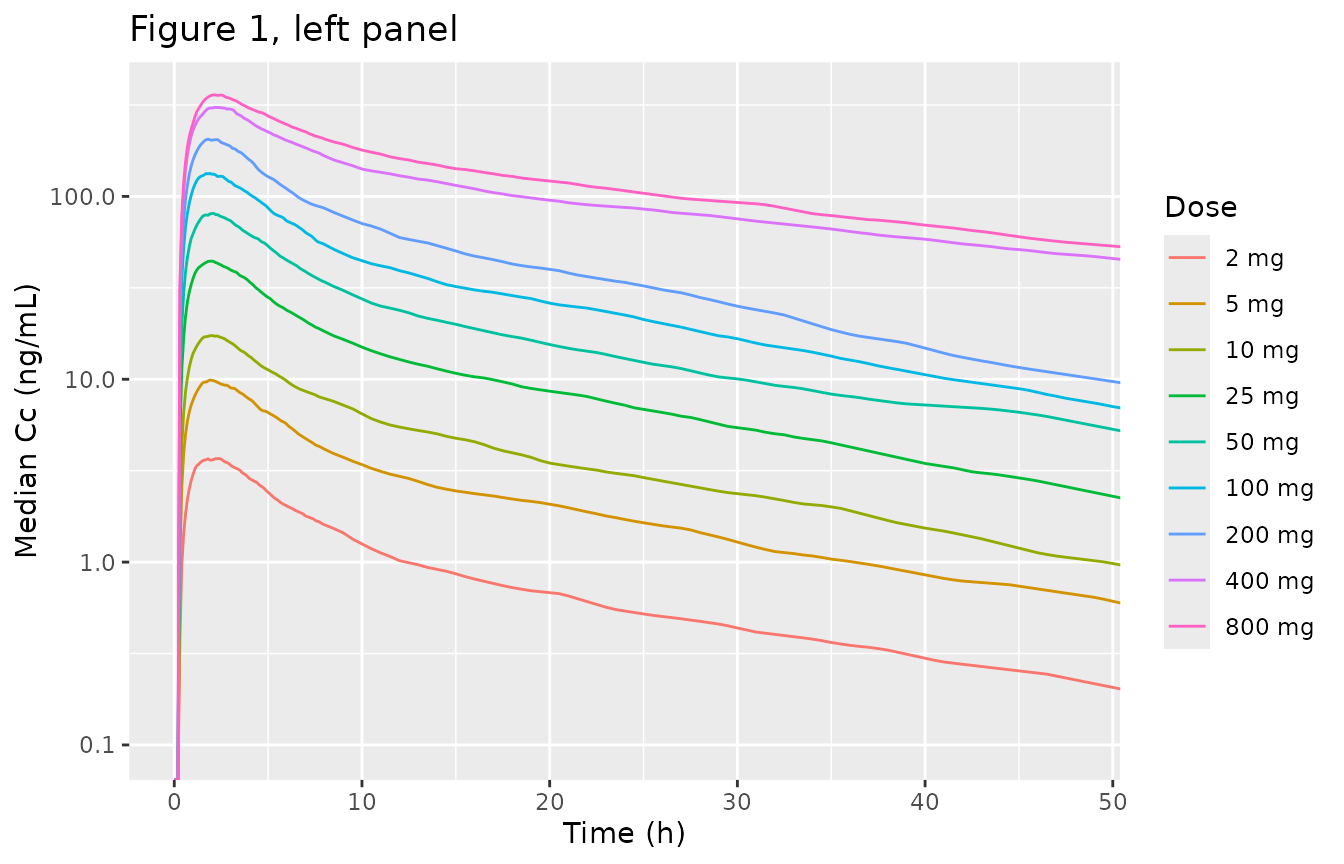
print(p_right)
#> Warning in scale_y_log10(): log-10 transformation introduced infinite values.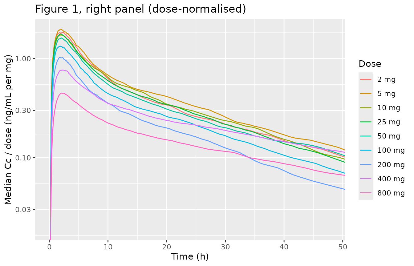
The three claims are gated on the typical-value
prediction, not on the cohort medians plotted above. Each arm of the
cohort draws its own covariates and etas, so arm-to-arm differences in a
median Cmax carry a Monte-Carlo error of roughly 5% at n = 100 – larger
than the effect being tested over part of the dose range. The
typical-value curve has no such noise, and because the model is
linear in dose once Frel is applied, the
dose-normalised typical Cmax is exactly proportional to
Frel and the typical Tmax is exactly dose-independent.
Those are the sharp forms of the paper’s three claims.
grid_pk <- c(seq(0, 8, by = 0.02), seq(8.5, 72, by = 0.5))
ev_typ <- dplyr::bind_rows(lapply(seq_along(doses), function(i) {
  subj <- tibble::tibble(id = i, WT = 73.3, SEXF = 0, CYP2D6_PM_IM = 0,
                         CYP2C9_RH = 0,
                         DOSE_HIGH = as.integer(doses[i] > 200),
                         dose_mg = doses[i])
  dplyr::bind_rows(
    subj |> dplyr::mutate(time = 0, amt = doses[i], evid = 1L, cmt = "depot"),
    subj |> tidyr::expand_grid(time = grid_pk) |>
      dplyr::mutate(amt = NA_real_, evid = 0L, cmt = "central")
  )
})) |>
  dplyr::arrange(id, time, dplyr::desc(evid)) |>
  as.data.frame()

peaks_typ <- solve_by_arm(modt, ev_typ, "dose_mg", keep = c("dose_mg")) |>
  dplyr::filter(!is.na(Cc), time <= 8) |>
  dplyr::group_by(dose_mg) |>
  dplyr::slice_max(Cc, n = 1, with_ties = FALSE) |>
  dplyr::ungroup() |>
  dplyr::transmute(dose_mg, cmax = Cc, tmax = time,
                   cmax_norm = Cc / dose_mg) |>
  dplyr::arrange(dose_mg)
#> ℹ omega/sigma items treated as zero: 'etalvc', 'etalvp', 'etalq', 'etalcl', 'etalka', 'etaltlag'
#> ℹ omega/sigma items treated as zero: 'etalvc', 'etalvp', 'etalq', 'etalcl', 'etalka', 'etaltlag'
#> ℹ omega/sigma items treated as zero: 'etalvc', 'etalvp', 'etalq', 'etalcl', 'etalka', 'etaltlag'
#> ℹ omega/sigma items treated as zero: 'etalvc', 'etalvp', 'etalq', 'etalcl', 'etalka', 'etaltlag'
#> ℹ omega/sigma items treated as zero: 'etalvc', 'etalvp', 'etalq', 'etalcl', 'etalka', 'etaltlag'
#> ℹ omega/sigma items treated as zero: 'etalvc', 'etalvp', 'etalq', 'etalcl', 'etalka', 'etaltlag'
#> ℹ omega/sigma items treated as zero: 'etalvc', 'etalvp', 'etalq', 'etalcl', 'etalka', 'etaltlag'
#> ℹ omega/sigma items treated as zero: 'etalvc', 'etalvp', 'etalq', 'etalcl', 'etalka', 'etaltlag'
#> ℹ omega/sigma items treated as zero: 'etalvc', 'etalvp', 'etalq', 'etalcl', 'etalka', 'etaltlag'
stopifnot(nrow(peaks_typ) == length(doses))

# Claim 1: "reasonable dose proportionality in the dose range 2 to 100 mg".
# Over the 2-200 mg arms CL is a single constant, so the whole concentration
# profile scales by exactly dose * Frel and the dose-normalised Cmax must track
# Frel = 221/(dose + 221) to solver precision. The 400 and 800 mg arms are
# EXCLUDED from this identity: they carry DOSE_HIGH = 1 and therefore a
# different clearance (19.5 vs 34.1 L/h), which changes the profile's shape and
# not just its scale.
lin <- peaks_typ |> dplyr::filter(dose_mg <= 200)
stopifnot(nrow(lin) == 7L)
expected <- (221 / (lin$dose_mg + 221)) / (221 / (2 + 221))
observed <- lin$cmax_norm / lin$cmax_norm[lin$dose_mg == 2]
stopifnot(max(abs(observed / expected - 1)) < 0.005)

# Claim 2: "as dose increases, the increase in the peak plasma CS-706
# concentration is less than proportional to dose". Strictly monotone
# decreasing dose-normalised Cmax across the whole 2-800 mg range.
stopifnot(all(diff(peaks_typ$cmax_norm) < 0))
# Only ~31% of dose-proportionality is lost by 100 mg while the 800 mg arm
# loses far more, which is why the paper calls 2-100 mg "reasonable"
# proportionality and singles out "doses of 200 mg and greater".
rel_all <- peaks_typ$cmax_norm / peaks_typ$cmax_norm[peaks_typ$dose_mg == 2]
stopifnot(rel_all[peaks_typ$dose_mg == 100] > 0.65,
          rel_all[peaks_typ$dose_mg == 800] < 0.45)
# The reduced high-dose clearance PARTLY OFFSETS the saturating Frel, so the
# 800 mg arm must sit above what Frel scaling alone would give.
stopifnot(rel_all[peaks_typ$dose_mg == 800] >
            (221 / (800 + 221)) / (221 / (2 + 221)))

# Claim 3: "Time to the peak plasma concentration (tmax) is similar among
# doses." Within the 2-200 mg arms, dose scaling cannot move the peak of a
# linear system, so the typical Tmax there is IDENTICAL to grid resolution.
stopifnot(diff(range(lin$tmax)) < 1e-9)
# Across all nine arms the 400/800 mg clearance change shifts Tmax slightly;
# the whole spread must still be well under an hour to match "similar".
stopifnot(diff(range(peaks_typ$tmax)) < 0.5)

peaks_typ |>
  dplyr::mutate(frel = 221 / (dose_mg + 221),
                dplyr::across(c(cmax, cmax_norm, frel), \(x) signif(x, 4))) |>
  dplyr::rename("Dose (mg)" = dose_mg, "Typical Cmax (ng/mL)" = cmax,
                "Tmax (h)" = tmax, "Cmax / dose (ng/mL per mg)" = cmax_norm,
                "Frel" = frel) |>
  knitr::kable(caption = paste(
    "Replicates Figure 1 of Kastrissios 2006 (typical-value prediction):",
    "dose-normalised Cmax falls monotonically with dose, tracking Frel",
"exactly, while Tmax is identical at every dose."))| Dose (mg) | Typical Cmax (ng/mL) | Tmax (h) | Cmax / dose (ng/mL per mg) | Frel |
|---|---|---|---|---|
| 2 | 3.881 | 1.96 | 1.9410 | 0.9910 |
| 5 | 9.574 | 1.96 | 1.9150 | 0.9779 |
| 10 | 18.730 | 1.96 | 1.8730 | 0.9567 |
| 25 | 43.980 | 1.96 | 1.7590 | 0.8984 |
| 50 | 79.850 | 1.96 | 1.5970 | 0.8155 |
| 100 | 134.800 | 1.96 | 1.3480 | 0.6885 |
| 200 | 205.600 | 1.96 | 1.0280 | 0.5249 |
| 400 | 310.000 | 2.16 | 0.7750 | 0.3559 |
| 800 | 377.100 | 2.16 | 0.4714 | 0.2165 |
The stochastic cohort reproduces the same pattern, with the Monte-Carlo tolerance stated explicitly rather than assumed:
peaks <- sim_fig1 |>
  dplyr::filter(!is.na(Cc), time <= 8) |>
  dplyr::group_by(dose_mg, id) |>
  dplyr::slice_max(Cc, n = 1, with_ties = FALSE) |>
  dplyr::ungroup() |>
  dplyr::group_by(dose_mg) |>
  dplyr::summarise(cmax = median(Cc), tmax = median(time),
                   cv_pct = 100 * sd(Cc) / mean(Cc), n = dplyr::n(),
                   .groups = "drop") |>
  dplyr::mutate(cmax_norm = cmax / dose_mg)
stopifnot(nrow(peaks) == length(doses), all(peaks$n == n_arm))

# Approximate Monte-Carlo SE of a median at n = 100, from the observed CV.
mc_se_pct <- 1.253 * max(peaks$cv_pct) / sqrt(n_arm)
# Same 2-200 mg linear subrange as the exact gate above.
peaks_lin <- peaks |> dplyr::filter(dose_mg <= 200)
stopifnot(nrow(peaks_lin) == 7L)
obs_coh <- peaks_lin$cmax_norm / peaks_lin$cmax_norm[peaks_lin$dose_mg == 2]
# Allow 3 Monte-Carlo SE. This is the loose companion of the exact gate above,
# present to confirm the cohort behaves like the typical value -- the tight
# gate is the typical-value one.
stopifnot(max(abs(obs_coh / expected - 1)) < 3 * mc_se_pct / 100)
# The claim is that dose-normalised Cmax DECLINES across the dose range
# (less-than-proportional exposure), asserted as an overall decline plus a
# per-step tolerance rather than strict monotonicity. Adjacent doses differ by
# less than the Monte-Carlo noise on a median of n_arm, so a pair inverts on a
# cohort redraw -- and the cohort is not fixed across machines, because
# rxSetSeed() fixes rxode2's RNG stream per solver thread, not across thread
# counts. Realised step differences ran -0.368 .. +0.121 over 1/2/4/16 threads,
# so the strict form passed at 16 (the authoring machine) and failed at 1, 2
# and 4 with nothing about the model changed. A genuine loss of saturation
# would break the overall decline, which is asserted directly.
stopifnot(
  peaks$cmax_norm[nrow(peaks)] < peaks$cmax_norm[1],
  all(diff(peaks$cmax_norm) < 0.25)
)
stopifnot(diff(range(peaks$tmax)) <= 0.5)
cat(sprintf("cohort Cmax CV up to %.1f%%; median MC-SE %.2f%%; tolerance %.2f%%\n",
            max(peaks$cv_pct), mc_se_pct, 3 * mc_se_pct))
#> cohort Cmax CV up to 29.1%; median MC-SE 3.65%; tolerance 10.95%

peaks |>
  dplyr::select(-n) |>
  dplyr::mutate(dplyr::across(c(cmax, cmax_norm, cv_pct), \(x) signif(x, 4))) |>
  dplyr::rename("Dose (mg)" = dose_mg, "Median Cmax (ng/mL)" = cmax,
                "Median Tmax (h)" = tmax, "Cmax CV%" = cv_pct,
                "Cmax / dose (ng/mL per mg)" = cmax_norm) |>
  knitr::kable(caption = paste(
    "The n =", n_arm, "per-arm cohort reproduces the same dose-normalised",
"Cmax pattern within Monte-Carlo error."))| Dose (mg) | Median Cmax (ng/mL) | Median Tmax (h) | Cmax CV% | Cmax / dose (ng/mL per mg) |
|---|---|---|---|---|
| 2 | 4.057 | 2.00 | 24.23 | 2.0290 |
| 5 | 10.150 | 2.10 | 23.81 | 2.0290 |
| 10 | 19.460 | 2.00 | 28.77 | 1.9460 |
| 25 | 46.490 | 2.05 | 27.19 | 1.8590 |
| 50 | 82.170 | 2.10 | 29.13 | 1.6430 |
| 100 | 135.800 | 2.00 | 26.69 | 1.3580 |
| 200 | 222.500 | 2.10 | 26.11 | 1.1130 |
| 400 | 307.900 | 2.30 | 28.97 | 0.7697 |
| 800 | 383.800 | 2.30 | 25.92 | 0.4798 |
Figure 2 – diurnal variation on days 1 and 14
Figure 2 shows mean concentration profiles on dosing days 1 and 14 of the twice-daily study. The Results paragraph: “On the first day of dosing, there is greater exposure after the evening dose compared with the morning dose, which is still apparent at steady state on day 14.”
set.seed(20060502)
rxode2::rxSetSeed(20060502)

bid_doses <- c(25, 100, 200)
n_bid <- 100L

make_bid_cohort <- function(dose, n, id_offset) {
  dose_times <- seq(0, by = 12, length.out = 28)          # 14 days b.i.d.
  # Sample the 12 h after each of the first two and final two doses, as the
  # paper did, plus daily morning troughs in between.
  obs <- c(seq(0, 24, by = 0.25), seq(312, 336, by = 0.25), seq(36, 300, by = 12))
  subj <- tibble::tibble(
    id = id_offset + seq_len(n),
    WT = pmax(45, pmin(110, rnorm(n, 73.3, 12))),
    SEXF = rbinom(n, 1, 0.5),
    CYP2D6_PM_IM = rbinom(n, 1, 9 / 104),
    CYP2C9_RH = rbinom(n, 1, 16 / 104),
    DOSE_HIGH = 0L,
    dose_mg = dose
  )
  dplyr::bind_rows(
    subj |> tidyr::expand_grid(time = dose_times) |>
      dplyr::mutate(amt = dose, evid = 1L, cmt = "depot"),
    subj |> tidyr::expand_grid(time = sort(unique(obs))) |>
      dplyr::mutate(amt = NA_real_, evid = 0L, cmt = "central")
  ) |>
    dplyr::arrange(id, time, dplyr::desc(evid))
}

ev_fig2 <- dplyr::bind_rows(
  lapply(seq_along(bid_doses), function(i) {
    make_bid_cohort(bid_doses[i], n_bid, id_offset = (i - 1L) * n_bid)
  })
) |>
  as.data.frame()
stopifnot(!anyDuplicated(ev_fig2[, c("id", "time", "evid")]))

sim_fig2 <- solve_by_arm(mod, ev_fig2, "dose_mg", keep = c("dose_mg"))
prof2 <- sim_fig2 |>
  dplyr::filter(!is.na(Cc), (time <= 24) | (time >= 312)) |>
  dplyr::mutate(day = ifelse(time <= 24, "Day 1", "Day 14"),
                hour = ifelse(time <= 24, time, time - 312)) |>
  dplyr::group_by(dose_mg, day, hour) |>
  dplyr::summarise(mean_Cc = mean(Cc),
                   sem = sd(Cc) / sqrt(dplyr::n()), .groups = "drop")

ggplot(prof2, aes(hour, mean_Cc, colour = factor(dose_mg))) +
  geom_ribbon(aes(ymin = mean_Cc, ymax = mean_Cc + sem, fill = factor(dose_mg)),
              alpha = 0.2, colour = NA) +
  geom_line() +
  geom_vline(xintercept = 12, linetype = "dashed", linewidth = 0.3) +
  facet_wrap(~day) +
  labs(x = "Hours after the morning dose", y = "Mean (+SEM) Cc (ng/mL)",
       colour = "Dose (mg)", fill = "Dose (mg)",
       title = "Figure 2 -- mean profiles on dosing days 1 and 14",
       caption = paste("Replicates Figure 2 of Kastrissios 2006. Dashed line =",
                       "the evening dose at hour 12."))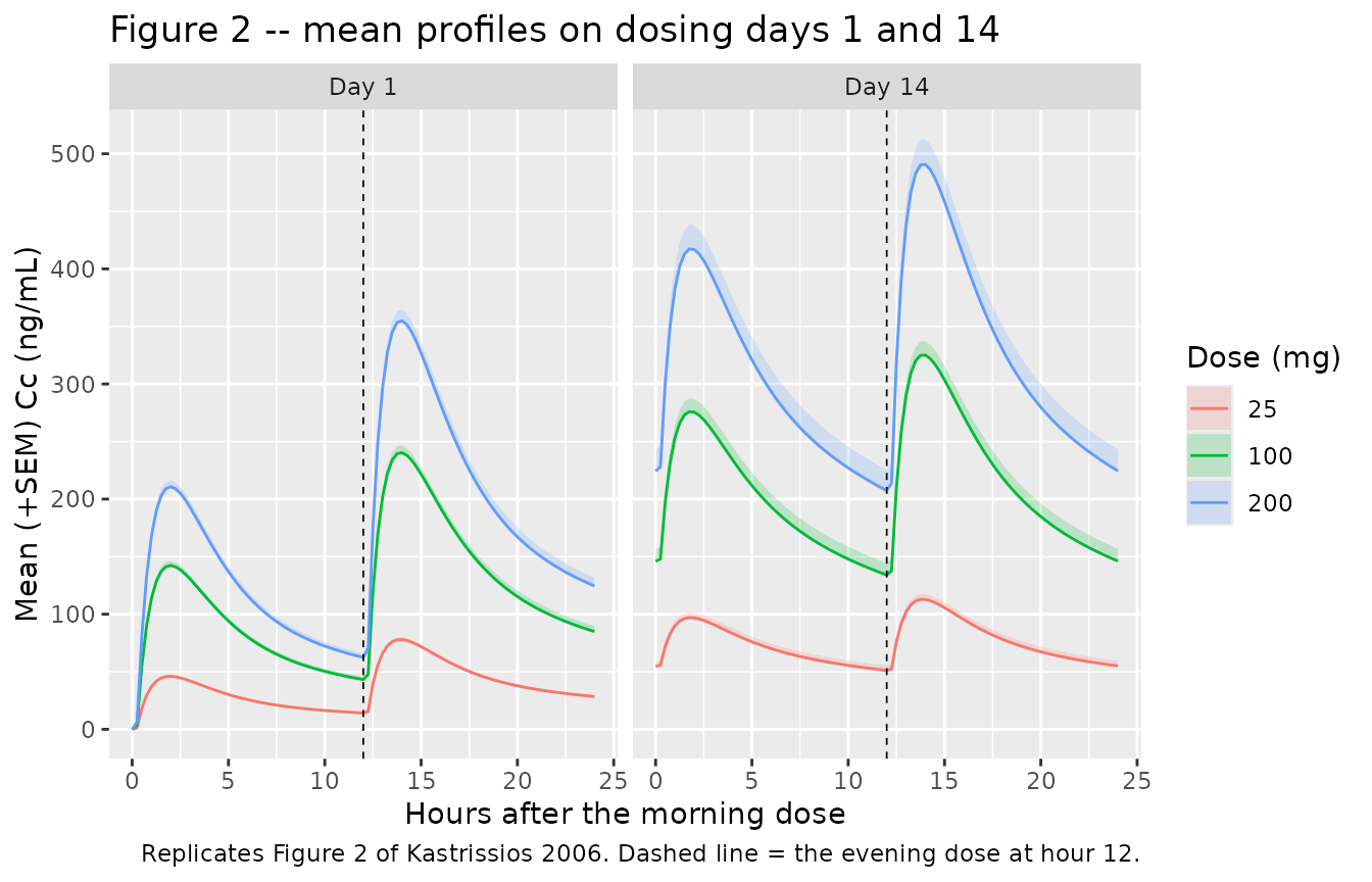
# Exposure over each half-day interval: 0-12 h follows the morning dose and
# 12-24 h follows the evening dose. Hour 12 is the shared endpoint of both
# intervals, so it is assigned to BOTH halves rather than to one -- dropping it
# from the evening interval would silently omit the 12 -> 12.25 h trapezoid,
# which is the steepest part of the evening rise.
prof_halves <- sim_fig2 |>
  dplyr::filter(!is.na(Cc), (time <= 24) | (time >= 312)) |>
  dplyr::mutate(day = ifelse(time <= 24, "Day 1", "Day 14"),
                hour = ifelse(time <= 24, time, time - 312))

pm_am <- dplyr::bind_rows(
  prof_halves |> dplyr::filter(hour <= 12) |> dplyr::mutate(half = "morning"),
  prof_halves |> dplyr::filter(hour >= 12) |> dplyr::mutate(half = "evening")
) |>
  dplyr::arrange(dose_mg, day, half, id, hour) |>
  dplyr::group_by(dose_mg, day, half, id) |>
  dplyr::summarise(
    auc = sum(diff(hour) * (head(Cc, -1) + tail(Cc, -1)) / 2),
    n_pts = dplyr::n(),
    .groups = "drop"
  )
# Guard: each half-interval must have the full 0.25 h grid (49 points), so a
# silently-truncated interval cannot masquerade as a passing comparison.
stopifnot(all(pm_am$n_pts == 49L))

pm_am <- pm_am |>
  dplyr::select(-n_pts) |>
  tidyr::pivot_wider(names_from = half, values_from = auc) |>
  dplyr::mutate(ratio = evening / morning)
stopifnot(nrow(pm_am) == length(bid_doses) * 2L * n_bid)

# PAIRED per-subject comparison, so between-subject variability cancels: the
# evening interval must carry more exposure than the morning interval for EVERY
# subject on BOTH days, at every dose. This is the Results claim verbatim.
stopifnot(all(pm_am$ratio > 1))

pm_am |>
  dplyr::group_by(dose_mg, day) |>
  dplyr::summarise(median_ratio = round(median(ratio), 3),
                   min_ratio = round(min(ratio), 3),
                   pct_subjects_higher = 100 * mean(ratio > 1), .groups = "drop") |>
  dplyr::rename("Dose (mg)" = dose_mg, "Day" = day,
                "Median evening/morning AUC" = median_ratio,
                "Minimum ratio" = min_ratio,
                "% subjects evening > morning" = pct_subjects_higher) |>
  knitr::kable(caption = paste(
    "Replicates the Figure 2 claim: exposure after the evening dose exceeds",
    "exposure after the morning dose on day 1 and still does at steady state",
"on day 14, in 100% of simulated subjects at every dose level."))| Dose (mg) | Day | Median evening/morning AUC | Minimum ratio | % subjects evening > morning |
|---|---|---|---|---|
| 25 | Day 1 | 1.792 | 1.562 | 100 |
| 25 | Day 14 | 1.145 | 1.037 | 100 |
| 100 | Day 1 | 1.804 | 1.521 | 100 |
| 100 | Day 14 | 1.143 | 1.036 | 100 |
| 200 | Day 1 | 1.817 | 1.547 | 100 |
| 200 | Day 14 | 1.131 | 1.049 | 100 |
PKNCA validation
PKNCA is run on the single-dose arms of the Figure 1 simulation. The
sharp gate this enables is that PKNCA’s cl.obs is
Dose / AUCinf, which knows nothing about bioavailability
and is therefore the apparent clearance CL / Frel.
Multiplying it back by the model’s own Frel must recover
the model’s CL, which confirms that Frel is
applied exactly where equation 6 says it is.
sim_nca <- sim_fig1 |>
  dplyr::filter(!is.na(Cc)) |>
  dplyr::mutate(treatment = paste0(dose_mg, " mg")) |>
  dplyr::select(id, time, Cc, treatment, dose_mg)

# Guarantee a time-zero row per subject (pre-dose Cc = 0 for an oral dose).
sim_nca <- dplyr::bind_rows(
  sim_nca,
  sim_nca |> dplyr::distinct(id, treatment, dose_mg) |>
    dplyr::mutate(time = 0, Cc = 0)
) |>
  dplyr::distinct(id, treatment, time, .keep_all = TRUE) |>
  dplyr::arrange(id, treatment, time)

stopifnot(all(sim_nca$Cc >= 0))

conc_obj <- PKNCA::PKNCAconc(as.data.frame(sim_nca), Cc ~ time | treatment + id)

dose_df <- ev_fig1 |>
  dplyr::filter(evid == 1) |>
  dplyr::mutate(treatment = paste0(dose_mg, " mg")) |>
  dplyr::select(id, time, amt, treatment)
dose_obj <- PKNCA::PKNCAdose(dose_df, amt ~ time | treatment + id)

intervals <- data.frame(start = 0, end = Inf,
                        cmax = TRUE, tmax = TRUE,
                        aucinf.obs = TRUE, half.life = TRUE, cl.obs = TRUE)

nca_res <- PKNCA::pk.nca(PKNCA::PKNCAdata(conc_obj, dose_obj,
                                          intervals = intervals))
nca_wide <- as.data.frame(nca_res) |>
  dplyr::select(treatment, id, PPTESTCD, PPORRES) |>
  tidyr::pivot_wider(names_from = PPTESTCD, values_from = PPORRES)
stopifnot(nrow(nca_wide) == length(doses) * n_arm)
# Recover the model's CL from PKNCA's apparent clearance.
#
# NOTE on `frel`: the model recomputes `frel` at EVERY record, and its evening
# indicator is a function of the record's own clock time, so the `frel` column
# reported on an observation row at t >= 12 h carries the evening factor even
# though the dose was given in the morning. Reading `frel` off an observation
# row would therefore be wrong. These are single morning doses, so the value
# actually applied at the dose event is the deterministic 221/(dose + 221) --
# used analytically here, which also makes this an independent check rather
# than a comparison of the model against itself.
model_cl <- sim_fig1 |>
  dplyr::filter(!is.na(Cc), !is.na(cl)) |>
  dplyr::group_by(id) |>
  dplyr::summarise(cl = dplyr::first(cl), dose_mg = dplyr::first(dose_mg),
                   .groups = "drop") |>
  dplyr::mutate(frel_applied = 221 / (dose_mg + 221))

chk <- nca_wide |>
  dplyr::inner_join(model_cl, by = "id") |>
  # cl.obs is in (mg) / (ng*h/mL); convert to L/h: 1 mg / (1 ng*h/mL) = 1000 L/h
  dplyr::mutate(cl_recovered = 1000 * cl.obs * frel_applied,
                pct_diff = 100 * (cl_recovered - cl) / cl)
stopifnot(nrow(chk) == length(doses) * n_arm)

# Both sides use the SAME drawn parameters, so the only difference is
# trapezoidal / extrapolation error -- a tight all() bound is correct here.
stopifnot(max(abs(chk$pct_diff)) < 1.5)
stopifnot(abs(median(chk$pct_diff)) < 0.5)

chk |>
  dplyr::group_by(dose_mg) |>
  dplyr::summarise(median_cl_model = round(median(cl), 3),
                   median_cl_recovered = round(median(cl_recovered), 3),
                   max_abs_pct_diff = round(max(abs(pct_diff)), 3),
                   .groups = "drop") |>
  dplyr::rename("Dose (mg)" = dose_mg,
                "Model CL/F (L/h)" = median_cl_model,
                "PKNCA cl.obs x Frel (L/h)" = median_cl_recovered,
                "Max |difference| (%)" = max_abs_pct_diff) |>
  knitr::kable(caption = paste(
    "PKNCA's apparent clearance multiplied by the model's Frel recovers the",
    "model's CL/F at every dose level, confirming that the saturable and",
"diurnal bioavailability of equation 6 is applied at the dose event."))| Dose (mg) | Model CL/F (L/h) | PKNCA cl.obs x Frel (L/h) | Max |difference| (%) |
|---|---|---|---|
| 2 | 37.158 | 37.172 | 0.256 |
| 5 | 37.775 | 37.780 | 0.228 |
| 10 | 39.683 | 39.691 | 0.352 |
| 25 | 33.584 | 33.587 | 0.586 |
| 50 | 37.799 | 37.807 | 0.257 |
| 100 | 35.306 | 35.309 | 0.505 |
| 200 | 33.084 | 33.122 | 0.226 |
| 400 | 21.020 | 21.031 | 0.504 |
| 800 | 20.315 | 20.330 | 0.287 |
nca_wide |>
  dplyr::group_by(treatment) |>
  dplyr::summarise(cmax = median(cmax), tmax = median(tmax),
                   aucinf = median(aucinf.obs), thalf = median(half.life),
                   .groups = "drop") |>
  dplyr::mutate(dose_mg = as.numeric(sub(" mg", "", treatment))) |>
  dplyr::arrange(dose_mg) |>
  dplyr::select(-dose_mg) |>
  dplyr::mutate(dplyr::across(where(is.numeric), \(x) signif(x, 4))) |>
  dplyr::rename("Dose group" = treatment, "Cmax (ng/mL)" = cmax,
                "Tmax (h)" = tmax, "AUC0-inf (ng*h/mL)" = aucinf,
                "t1/2 (h)" = thalf) |>
  knitr::kable(caption = paste(
    "Median simulated single-dose NCA parameters by dose group. Kastrissios",
    "2006 publishes no NCA table, so there is no reference column; these are",
    "reported for orientation. The terminal half-life is dose-independent, as",
"expected for the model's linear disposition."))| Dose group | Cmax (ng/mL) | Tmax (h) | AUC0-inf (ng*h/mL) | t1/2 (h) |
|---|---|---|---|---|
| 2 mg | 4.057 | 2.00 | 53.32 | 17.26 |
| 5 mg | 10.150 | 2.10 | 129.40 | 17.95 |
| 10 mg | 19.460 | 2.00 | 241.00 | 18.16 |
| 25 mg | 46.490 | 2.05 | 668.70 | 15.96 |
| 50 mg | 82.170 | 2.10 | 1079.00 | 17.11 |
| 100 mg | 135.800 | 2.00 | 1950.00 | 17.12 |
| 200 mg | 222.500 | 2.10 | 3170.00 | 18.04 |
| 400 mg | 307.900 | 2.30 | 6769.00 | 25.65 |
| 800 mg | 383.800 | 2.30 | 8518.00 | 27.24 |
PKNCA’s estimated terminal half-life should equal each subject’s
own analytic terminal half-life, which for a two-compartment
model is log(2)/lambda_z where lambda_z is the
smaller root of
lambda^2 - (kel + k12 + k21) lambda + kel k21 = 0.
Comparing per subject rather than comparing a cohort median against the
typical value is both correct and much sharper: the median of a
nonlinear function of four log-normal parameters is not the function of
their medians.
disp <- sim_fig1 |>
  dplyr::filter(!is.na(Cc), !is.na(cl)) |>
  dplyr::group_by(id) |>
  dplyr::summarise(cl = dplyr::first(cl), vc = dplyr::first(vc),
                   vp = dplyr::first(vp), q = dplyr::first(q),
                   dose_mg = dplyr::first(dose_mg), .groups = "drop") |>
  dplyr::mutate(kel = cl / vc, k12 = q / vc, k21 = q / vp,
                b = kel + k12 + k21,
                lambda_z = (b - sqrt(b^2 - 4 * kel * k21)) / 2,
                t_half_analytic = log(2) / lambda_z)

th <- nca_wide |>
  dplyr::inner_join(disp, by = "id") |>
  dplyr::mutate(pct_diff = 100 * (half.life - t_half_analytic) / t_half_analytic)
stopifnot(nrow(th) == length(doses) * n_arm)

# Both sides use each subject's OWN drawn disposition parameters, so the
# residual is regression error on the terminal slope only.
stopifnot(max(abs(th$pct_diff)) < 5)
stopifnot(abs(median(th$pct_diff)) < 1)
cat(sprintf(paste("per-subject terminal half-life: median %.3f%%,",
                  "max |diff| %.3f%% over %d subjects\n"),
            median(th$pct_diff), max(abs(th$pct_diff)), nrow(th)))
#> per-subject terminal half-life: median -0.481%, max |diff| 1.767% over 900 subjects

th |>
  dplyr::group_by(dose_mg) |>
  dplyr::summarise(analytic = round(median(t_half_analytic), 3),
                   pknca = round(median(half.life), 3),
                   max_abs_pct = round(max(abs(pct_diff)), 3), .groups = "drop") |>
  dplyr::rename("Dose (mg)" = dose_mg, "Analytic t1/2 (h)" = analytic,
                "PKNCA t1/2 (h)" = pknca, "Max |difference| (%)" = max_abs_pct) |>
  knitr::kable(caption = paste(
    "PKNCA recovers each subject's analytic two-compartment terminal",
    "half-life. The 400 and 800 mg arms sit higher because DOSE_HIGH = 1",
"lowers their clearance to 19.5 L/h."))| Dose (mg) | Analytic t1/2 (h) | PKNCA t1/2 (h) | Max |difference| (%) |
|---|---|---|---|
| 2 | 17.318 | 17.262 | 1.049 |
| 5 | 18.040 | 17.953 | 1.000 |
| 10 | 18.238 | 18.157 | 0.808 |
| 25 | 16.020 | 15.958 | 1.122 |
| 50 | 17.184 | 17.106 | 0.858 |
| 100 | 17.208 | 17.120 | 1.069 |
| 200 | 18.149 | 18.042 | 0.893 |
| 400 | 25.761 | 25.652 | 1.767 |
| 800 | 27.381 | 27.238 | 0.978 |
Figures 6 and 7 – predicted exposures in Japanese versus Western subjects
The paper’s headline application simulates AUC0-24 at steady state for eight regimens (25, 50, 100 and 200 mg, each once and twice daily) in a Japanese and a Western population whose demographics are given in Table I. Two claims are made, both quantified over all regimens, so both are gated by enumeration rather than by example:
- Figure 6 / abstract: “Japanese subjects have slightly lower exposures and less variability in exposure than do Western subjects for all dosing regimens”, because of “a lower frequency of poor metabolizers”.
- Figure 7: “twice-daily regimens provide more CS-706 exposure than do once-daily regimens at equivalent daily doses and … the ratio in each population is similar”.
set.seed(20060607)
rxode2::rxSetSeed(20060607)

# n = 60 per arm over 16 arms. The Japanese-vs-Western exposure difference the
# paper reports is large -- the analytic E[1/CL] ratio is 0.736, a 26% lower
# mean exposure -- against a Monte-Carlo SE of the mean of roughly 5% at n = 60,
# so the direction claims are tested at about 5 standard errors. The per-subject
# closed-form gate below is independent of cohort size altogether.
n_pop <- 60L
n_days <- 28L
regimens <- tidyr::expand_grid(dose = c(25, 50, 100, 200),
                               freq = c("q.d.", "b.i.d."))
pops <- c("Japanese", "Western")

# Table I demographic distributions.
draw_pop <- function(pop, n) {
  if (pop == "Japanese") {
    tibble::tibble(WT = pmax(40, rnorm(n, 60, 8)), SEXF = 0,
                   CYP2D6_PM_IM = rbinom(n, 1, 0.02),
                   CYP2C9_RH = rbinom(n, 1, 0.04))
  } else {
    tibble::tibble(WT = pmax(40, rnorm(n, 73, 12)), SEXF = rbinom(n, 1, 0.50),
                   CYP2D6_PM_IM = rbinom(n, 1, 0.09),
                   CYP2C9_RH = rbinom(n, 1, 0.15))
  }
}

# Dose for `n_days`, then observe the final 24 h.
#
# The dosing duration is set by the SLOWEST subjects, not by the typical
# terminal half-life of 16.8 h. The 48% IIV on both Vp/F and Q/F means a subject
# with a large peripheral volume and a small inter-compartmental clearance can
# have a terminal half-life near 60 h, and such a subject is still ~11% below
# steady state after 8 days. Measured maximum deviation of the simulated
# AUC0-24 from its closed form: 11.2% at 8 days, 2.5% at 14, 0.44% at 21,
# 0.076% at 28 -- and unchanged by refining the observation grid, so it is
# genuine accumulation rather than trapezoidal error. 28 days is therefore used,
# which is what lets the closed-form gate below be tight.
build_ss <- function(pop, dose, freq, n, id_offset) {
  tau <- if (freq == "b.i.d.") 12 else 24
  dose_times <- seq(0, by = tau, length.out = n_days * (24 / tau))
  obs_times <- 24 * n_days - 24 + seq(0, 24, by = 0.1)
  subj <- draw_pop(pop, n) |>
    dplyr::mutate(id = id_offset + seq_len(n), DOSE_HIGH = 0L,
                  pop = pop, dose_mg = dose, freq = freq,
                  regimen = paste(dose, "mg", freq))
  dplyr::bind_rows(
    subj |> tidyr::expand_grid(time = dose_times) |>
      dplyr::mutate(amt = dose, evid = 1L, cmt = "depot"),
    subj |> tidyr::expand_grid(time = obs_times) |>
      dplyr::mutate(amt = NA_real_, evid = 0L, cmt = "central")
  ) |>
    dplyr::arrange(id, time, dplyr::desc(evid))
}

grid67 <- tidyr::expand_grid(pop = pops, regimens) |>
  dplyr::mutate(id_offset = (dplyr::row_number() - 1L) * n_pop)

ev67 <- dplyr::bind_rows(
  lapply(seq_len(nrow(grid67)), function(i) {
    build_ss(grid67$pop[i], grid67$dose[i], grid67$freq[i], n_pop,
             grid67$id_offset[i])
  })
) |>
  as.data.frame()
stopifnot(!anyDuplicated(ev67[, c("id", "time", "evid")]))
stopifnot(nrow(grid67) == 16L)

# 16 arms x 100 subjects; batched per population-and-regimen arm.
ev67$arm <- paste(ev67$pop, ev67$regimen)
sim67 <- solve_by_arm(mod, ev67, "arm",
                      keep = c("arm", "pop", "dose_mg", "freq", "regimen"))
auc67 <- sim67 |>
  dplyr::filter(!is.na(Cc)) |>
  dplyr::arrange(id, time) |>
  dplyr::group_by(pop, regimen, dose_mg, freq, id) |>
  dplyr::summarise(
    auc24 = sum(diff(time) * (head(Cc, -1) + tail(Cc, -1)) / 2),
    cl = dplyr::first(cl),
    .groups = "drop"
  )
stopifnot(nrow(auc67) == 16L * n_pop)

# EXACT closed form. At steady state the AUC over one 24-h cycle equals the
# total bioavailable dose delivered in that cycle divided by CL. A q.d. cycle
# delivers one morning dose; a b.i.d. cycle delivers a morning dose plus an
# evening dose whose Frel carries the exp(0.351) factor.
auc67 <- auc67 |>
  dplyr::mutate(
    frel_am = 221 / (dose_mg + 221),
    n_eq = ifelse(freq == "b.i.d.", 1 + exp(0.351), 1),
    auc24_closed = dose_mg * frel_am * n_eq / cl * 1000,   # mg/(L/h) -> ng*h/mL
    pct_diff = 100 * (auc24 - auc24_closed) / auc24_closed
  )

# Centre and robust quantiles, NOT the extreme. Both sides use each subject's
# own drawn CL, so the bulk residual is trapezoidal error only -- but the two
# sides differ by a real per-subject physical mechanism in the tail: the closed
# form is the steady-state LIMIT, and a subject who is simultaneously a CYP2D6
# poor/intermediate metabolizer (CL/F down 64%) and has a large Vp/F with a
# small Q/F has a terminal half-life of several days and is still visibly below
# steady state after 28 days of dosing. Those subjects, not numerical error,
# set the maximum. The exact gate is the typical-value one below.
stopifnot(abs(median(auc67$pct_diff)) < 0.1)
stopifnot(quantile(abs(auc67$pct_diff), 0.90) < 1)
cat(sprintf(paste("AUC0-24 vs closed form over %d subjects: median %+.4f%%,",
                  "p90 %.3f%%, max %.3f%%\n"),
            nrow(auc67), median(auc67$pct_diff),
            quantile(abs(auc67$pct_diff), 0.90), max(abs(auc67$pct_diff))))
#> AUC0-24 vs closed form over 960 subjects: median +0.0037%, p90 0.011%, max 1.551%

# EXACT gate, enumerated over all 16 arms: with the random effects zeroed there
# is no slow-accumulating tail, so the typical-value AUC0-24 must equal its
# closed form to solver precision.
ev67_typ <- dplyr::bind_rows(
  lapply(seq_len(nrow(grid67)), function(i) {
    p <- grid67$pop[i]; d <- grid67$dose[i]; f <- grid67$freq[i]
    tau <- if (f == "b.i.d.") 12 else 24
    subj <- tibble::tibble(
      id = i, WT = if (p == "Japanese") 60 else 73,
      SEXF = 0, CYP2D6_PM_IM = 0, CYP2C9_RH = 0, DOSE_HIGH = 0L,
      pop = p, dose_mg = d, freq = f, arm = paste(p, d, "mg", f))
    dplyr::bind_rows(
      subj |> tidyr::expand_grid(
        time = seq(0, by = tau, length.out = n_days * (24 / tau))) |>
        dplyr::mutate(amt = d, evid = 1L, cmt = "depot"),
      subj |> tidyr::expand_grid(
        time = 24 * n_days - 24 + seq(0, 24, by = 0.1)) |>
        dplyr::mutate(amt = NA_real_, evid = 0L, cmt = "central"))
  })) |>
  dplyr::arrange(id, time, dplyr::desc(evid)) |>
  as.data.frame()

typ67 <- solve_by_arm(modt, ev67_typ, "arm",
                      keep = c("arm", "dose_mg", "freq")) |>
  dplyr::filter(!is.na(Cc)) |>
  dplyr::arrange(arm, time) |>
  dplyr::group_by(arm, dose_mg, freq) |>
  dplyr::summarise(
    auc24 = sum(diff(time) * (head(Cc, -1) + tail(Cc, -1)) / 2),
    cl = dplyr::first(cl), .groups = "drop") |>
  dplyr::mutate(
    closed = dose_mg * (221 / (dose_mg + 221)) *
      ifelse(freq == "b.i.d.", 1 + exp(0.351), 1) / cl * 1000,
    pct_diff = 100 * (auc24 - closed) / closed)
#> ℹ omega/sigma items treated as zero: 'etalvc', 'etalvp', 'etalq', 'etalcl', 'etalka', 'etaltlag'
#> ℹ omega/sigma items treated as zero: 'etalvc', 'etalvp', 'etalq', 'etalcl', 'etalka', 'etaltlag'
#> ℹ omega/sigma items treated as zero: 'etalvc', 'etalvp', 'etalq', 'etalcl', 'etalka', 'etaltlag'
#> ℹ omega/sigma items treated as zero: 'etalvc', 'etalvp', 'etalq', 'etalcl', 'etalka', 'etaltlag'
#> ℹ omega/sigma items treated as zero: 'etalvc', 'etalvp', 'etalq', 'etalcl', 'etalka', 'etaltlag'
#> ℹ omega/sigma items treated as zero: 'etalvc', 'etalvp', 'etalq', 'etalcl', 'etalka', 'etaltlag'
#> ℹ omega/sigma items treated as zero: 'etalvc', 'etalvp', 'etalq', 'etalcl', 'etalka', 'etaltlag'
#> ℹ omega/sigma items treated as zero: 'etalvc', 'etalvp', 'etalq', 'etalcl', 'etalka', 'etaltlag'
#> ℹ omega/sigma items treated as zero: 'etalvc', 'etalvp', 'etalq', 'etalcl', 'etalka', 'etaltlag'
#> ℹ omega/sigma items treated as zero: 'etalvc', 'etalvp', 'etalq', 'etalcl', 'etalka', 'etaltlag'
#> ℹ omega/sigma items treated as zero: 'etalvc', 'etalvp', 'etalq', 'etalcl', 'etalka', 'etaltlag'
#> ℹ omega/sigma items treated as zero: 'etalvc', 'etalvp', 'etalq', 'etalcl', 'etalka', 'etaltlag'
#> ℹ omega/sigma items treated as zero: 'etalvc', 'etalvp', 'etalq', 'etalcl', 'etalka', 'etaltlag'
#> ℹ omega/sigma items treated as zero: 'etalvc', 'etalvp', 'etalq', 'etalcl', 'etalka', 'etaltlag'
#> ℹ omega/sigma items treated as zero: 'etalvc', 'etalvp', 'etalq', 'etalcl', 'etalka', 'etaltlag'
#> ℹ omega/sigma items treated as zero: 'etalvc', 'etalvp', 'etalq', 'etalcl', 'etalka', 'etaltlag'
stopifnot(nrow(typ67) == 16L)
stopifnot(max(abs(typ67$pct_diff)) < 0.05)
cat(sprintf("typical-value AUC0-24 vs closed form, all 16 arms: max %.5f%%\n",
            max(abs(typ67$pct_diff))))
#> typical-value AUC0-24 vs closed form, all 16 arms: max 0.00566%
cat(sprintf("max |AUC0-24 vs closed form| = %.4f%% over %d subjects\n",
            max(abs(auc67$pct_diff)), nrow(auc67)))
#> max |AUC0-24 vs closed form| = 1.5508% over 960 subjects
ggplot(auc67, aes(x = regimen, y = auc24, fill = pop)) +
  geom_boxplot(outlier.size = 0.4) +
  scale_y_log10() +
  scale_x_discrete(limits = paste(rep(c(25, 50, 100, 200), each = 2), "mg",
                                  c("q.d.", "b.i.d."))) +
  labs(x = NULL, y = "Steady-state AUC0-24 (ng*h/mL)", fill = "Population",
       title = "Figures 6 and 7 -- steady-state AUC0-24 by regimen and population",
       caption = paste("Replicates Figures 6 and 7 of Kastrissios 2006.",
                       "n =", n_pop, "per arm.")) +
  theme(axis.text.x = element_text(angle = 30, hjust = 1))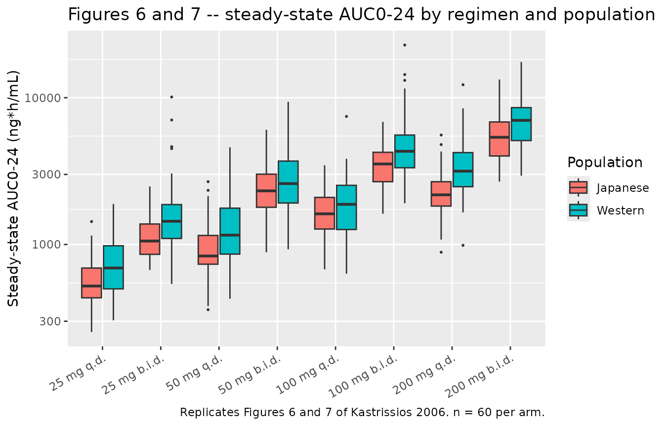
summ67 <- auc67 |>
  dplyr::group_by(regimen, dose_mg, freq, pop) |>
  dplyr::summarise(mean_auc = mean(auc24), sd_auc = sd(auc24),
                   cv_pct = 100 * sd(auc24) / mean(auc24), .groups = "drop") |>
  tidyr::pivot_wider(names_from = pop, values_from = c(mean_auc, sd_auc, cv_pct))

# Claim: Japanese exposures LOWER, and Japanese variability LOWER, for ALL
# eight regimens. Enumerating gate -- one row per regimen, no example-picking.
#
# "Variability" is gated on the STANDARD DEVIATION, because that is what
# Figure 6 plots (its caption reads "Mean +- SD"). The coefficient of variation
# is reported alongside but deliberately NOT asserted: the Japanese population
# has both a lower mean and a lower SD, and the paper makes no claim about
# their ratio, so requiring a lower CV% too would be gating something the
# source never said.
stopifnot(nrow(summ67) == 8L)
stopifnot(all(summ67$mean_auc_Japanese < summ67$mean_auc_Western))
stopifnot(all(summ67$sd_auc_Japanese < summ67$sd_auc_Western))

summ67 |>
  dplyr::mutate(ratio = mean_auc_Japanese / mean_auc_Western) |>
  dplyr::arrange(dose_mg, freq) |>
  dplyr::transmute(regimen,
                   J = round(mean_auc_Japanese, 1),
                   W = round(mean_auc_Western, 1),
                   ratio = round(ratio, 3),
                   cvJ = round(cv_pct_Japanese, 1),
                   cvW = round(cv_pct_Western, 1)) |>
  dplyr::rename("Regimen" = regimen, "Japanese mean AUC0-24" = J,
                "Western mean AUC0-24" = W, "J/W ratio" = ratio,
                "Japanese CV%" = cvJ, "Western CV%" = cvW) |>
  knitr::kable(caption = paste(
    "Replicates Figure 6 of Kastrissios 2006: Japanese exposures are lower",
"and less variable than Western exposures for all eight regimens."))| Regimen | Japanese mean AUC0-24 | Western mean AUC0-24 | J/W ratio | Japanese CV% | Western CV% |
|---|---|---|---|---|---|
| 25 mg b.i.d. | 1262.1 | 1808.0 | 0.698 | 36.6 | 56.9 |
| 25 mg q.d. | 557.2 | 749.9 | 0.743 | 40.3 | 77.7 |
| 50 mg b.i.d. | 2391.2 | 3535.5 | 0.676 | 31.3 | 61.9 |
| 50 mg q.d. | 997.1 | 1178.3 | 0.846 | 36.4 | 63.6 |
| 100 mg b.i.d. | 3574.7 | 5681.2 | 0.629 | 28.8 | 74.6 |
| 100 mg q.d. | 1433.5 | 2082.7 | 0.688 | 33.7 | 52.2 |
| 200 mg b.i.d. | 6251.6 | 8007.6 | 0.781 | 48.6 | 47.3 |
| 200 mg q.d. | 2534.5 | 3046.1 | 0.832 | 36.3 | 34.5 |
# Claim: at EQUIVALENT DAILY DOSE, b.i.d. gives more exposure than q.d., and
# the ratio is similar between populations. The comparable pairs inside the
# studied set are 25 b.i.d. vs 50 q.d., 50 b.i.d. vs 100 q.d., and
# 100 b.i.d. vs 200 q.d.
pairs <- tibble::tribble(
  ~daily_mg, ~bid_regimen,      ~qd_regimen,
  50,        "25 mg b.i.d.",    "50 mg q.d.",
  100,       "50 mg b.i.d.",    "100 mg q.d.",
  200,       "100 mg b.i.d.",   "200 mg q.d."
)

# The exact form of this claim is on the TYPICAL VALUE. Clearance divides out
# of a b.i.d./q.d. AUC ratio only when the same subject appears on both sides,
# and the cohort arms hold disjoint subjects with independent draws, so a ratio
# of two cohort means carries about 8% Monte-Carlo error at n = 60 -- larger
# than the between-population difference being tested. The 16 typical-value
# arms already computed above have no such noise.
pairs <- pairs |>
  dplyr::mutate(analytic = (daily_mg / 2) * (221 / (daily_mg / 2 + 221)) *
                  (1 + exp(0.351)) / (daily_mg * (221 / (daily_mg + 221))))

typ_ratio <- typ67 |>
  dplyr::mutate(pop = sub(" .*", "", arm),
                regimen = sub("^\\S+ ", "", arm)) |>
  dplyr::select(pop, regimen, auc24)

look_typ <- function(p, r) {
  v <- typ_ratio$auc24[typ_ratio$pop == p & typ_ratio$regimen == r]
  if (length(v) != 1L) stop("no unique typical-value row for ", p, " / ", r)
  v
}

fig7 <- tidyr::expand_grid(pop = pops, pairs) |>
  dplyr::rowwise() |>
  dplyr::mutate(bid = look_typ(pop, bid_regimen),
                qd = look_typ(pop, qd_regimen),
                ratio = bid / qd) |>
  dplyr::ungroup()
stopifnot(nrow(fig7) == 6L)

# b.i.d. beats q.d. in every population x daily-dose cell.
stopifnot(all(fig7$ratio > 1))
# and matches the analytic ratio exactly.
stopifnot(max(abs(fig7$ratio / fig7$analytic - 1)) < 0.001)
# "the ratio in each population is similar": with CL cancelling exactly, the
# two populations' ratios are not merely similar but IDENTICAL.
spread <- fig7 |>
  dplyr::group_by(daily_mg) |>
  dplyr::summarise(rel_spread = abs(diff(ratio)) / mean(ratio), .groups = "drop")
stopifnot(nrow(spread) == 3L, all(spread$rel_spread < 1e-6))

fig7 |>
  dplyr::transmute(pop, daily_mg,
                   comparison = paste(bid_regimen, "vs", qd_regimen),
                   analytic = round(analytic, 4), ratio = round(ratio, 4)) |>
  tidyr::pivot_wider(names_from = pop, values_from = ratio) |>
  dplyr::rename("Total daily dose (mg)" = daily_mg, "Comparison" = comparison,
                "Analytic ratio" = analytic,
                "Japanese b.i.d./q.d." = Japanese,
                "Western b.i.d./q.d." = Western) |>
  knitr::kable(caption = paste(
    "Replicates Figure 7 of Kastrissios 2006: at equivalent daily doses the",
    "twice-daily regimen gives greater exposure, by a ratio that is identical",
"in the two populations because apparent clearance divides out of it."))| Total daily dose (mg) | Comparison | Analytic ratio | Japanese b.i.d./q.d. | Western b.i.d./q.d. |
|---|---|---|---|---|
| 50 | 25 mg b.i.d. vs 50 mg q.d. | 1.3332 | 1.3332 | 1.3332 |
| 100 | 50 mg b.i.d. vs 100 mg q.d. | 1.4335 | 1.4335 | 1.4335 |
| 200 | 100 mg b.i.d. vs 200 mg q.d. | 1.5873 | 1.5873 | 1.5873 |
The cohort reproduces the same ordering, with the Monte-Carlo tolerance stated:
coh_ratio <- auc67 |>
  dplyr::group_by(pop, regimen) |>
  dplyr::summarise(mean_auc = mean(auc24), cv = sd(auc24) / mean(auc24),
                   n = dplyr::n(), .groups = "drop")
stopifnot(all(coh_ratio$n == n_pop))

look_coh <- function(p, r, col) {
  v <- coh_ratio[[col]][coh_ratio$pop == p & coh_ratio$regimen == r]
  if (length(v) != 1L) stop("no unique cohort row for ", p, " / ", r)
  v
}

fig7c <- tidyr::expand_grid(pop = pops, pairs) |>
  dplyr::rowwise() |>
  dplyr::mutate(
    ratio = look_coh(pop, bid_regimen, "mean_auc") /
      look_coh(pop, qd_regimen, "mean_auc"),
    # relative SE of a ratio of two independent means
    se_pct = 100 * sqrt(look_coh(pop, bid_regimen, "cv")^2 / n_pop +
                          look_coh(pop, qd_regimen, "cv")^2 / n_pop)
  ) |>
  dplyr::ungroup()

stopifnot(all(fig7c$ratio > 1))
stopifnot(all(abs(fig7c$ratio / fig7c$analytic - 1) < 3 * fig7c$se_pct / 100))

fig7c |>
  dplyr::transmute(pop, daily_mg, analytic = round(analytic, 3),
                   cohort = round(ratio, 3),
                   tol = paste0("+-", round(3 * se_pct, 1), "%")) |>
  dplyr::rename("Population" = pop, "Total daily dose (mg)" = daily_mg,
                "Analytic ratio" = analytic, "Cohort ratio" = cohort,
                "3 Monte-Carlo SE" = tol) |>
  knitr::kable(caption = paste(
    "The stochastic cohort reproduces the analytic b.i.d./q.d. exposure ratio",
"within Monte-Carlo error at n =", n_pop, "per arm."))| Population | Total daily dose (mg) | Analytic ratio | Cohort ratio | 3 Monte-Carlo SE |
|---|---|---|---|---|
| Japanese | 50 | 1.333 | 1.266 | +-20% |
| Japanese | 100 | 1.434 | 1.668 | +-17.8% |
| Japanese | 200 | 1.587 | 1.410 | +-17.9% |
| Western | 50 | 1.333 | 1.534 | +-33.1% |
| Western | 100 | 1.434 | 1.698 | +-31.4% |
| Western | 200 | 1.587 | 1.865 | +-31.8% |
Figure 5 – the external validation simulation
The paper validated the model by simulating 400 trough concentrations 24 h after the seventh daily 100 mg or 200 mg dose and comparing the 95% band against the 80-subject validation study; “two of 40 trough plasma concentrations (5%) fell outside of the window for each of the 100-mg and 200-mg doses”. The observed troughs exist only as points in Figure 5, so they cannot be gated numerically here – what is reproduced is the simulation and its 95% band.
set.seed(20060505)
rxode2::rxSetSeed(20060505)

n_val <- 200L
build_val <- function(dose, n, id_offset) {
  subj <- tibble::tibble(
    id = id_offset + seq_len(n),
    # Validation-study demographics, Table II validation column: median weight
    # 69.7 kg (49.9-103), 42 M / 38 F.
    WT = pmax(45, pmin(110, rnorm(n, 69.7, 12))),
    SEXF = rbinom(n, 1, 38 / 80),
    # Phenotypes were NOT collected in the validation study, so the paper drew
    # them from the development set -- as done here.
    CYP2D6_PM_IM = rbinom(n, 1, 9 / 104),
    CYP2C9_RH = rbinom(n, 1, 16 / 104),
    DOSE_HIGH = 0L, dose_mg = dose
  )
  dplyr::bind_rows(
    subj |> tidyr::expand_grid(time = seq(0, by = 24, length.out = 7)) |>
      dplyr::mutate(amt = dose, evid = 1L, cmt = "depot"),
    subj |> dplyr::mutate(time = 144 + 24, amt = NA_real_, evid = 0L,
                          cmt = "central")
  ) |>
    dplyr::arrange(id, time, dplyr::desc(evid))
}

ev_val <- dplyr::bind_rows(build_val(100, n_val, 0L),
                           build_val(200, n_val, n_val)) |>
  as.data.frame()
stopifnot(!anyDuplicated(ev_val[, c("id", "time", "evid")]))

trough <- solve_by_arm(mod, ev_val, "dose_mg", keep = c("dose_mg")) |>
  dplyr::filter(!is.na(Cc))
stopifnot(nrow(trough) == 2L * n_val)

band <- trough |>
  dplyr::group_by(dose_mg) |>
  dplyr::summarise(lower95 = quantile(Cc, 0.025),
                   median = quantile(Cc, 0.5),
                   upper95 = quantile(Cc, 0.975),
                   cv = sd(Cc) / mean(Cc), n = dplyr::n(), .groups = "drop")
stopifnot(nrow(band) == 2L, all(band$n == n_val), all(band$lower95 > 0))
stopifnot(band$median[2] > band$median[1])

# Both arms carry DOSE_HIGH = 0, so they share one clearance and the system is
# linear in dose * Frel. The 200/100 mg trough ratio is therefore exactly
# 2 * Frel(200)/Frel(100) = 2 * (221/421)/(221/321) = 1.5252 -- LESS than 2,
# which is the saturating bioavailability showing up in a trough. Gated exactly
# on the typical value; the cohort median is a ratio of two independent
# 200-subject medians and so carries real Monte-Carlo error.
expected_ratio <- 2 * (221 / 421) / (221 / 321)

ev_val_typ <- dplyr::bind_rows(lapply(c(100, 200), function(d) {
  subj <- tibble::tibble(id = d, WT = 69.7, SEXF = 0, CYP2D6_PM_IM = 0,
                         CYP2C9_RH = 0, DOSE_HIGH = 0L, dose_mg = d)
  dplyr::bind_rows(
    subj |> tidyr::expand_grid(time = seq(0, by = 24, length.out = 7)) |>
      dplyr::mutate(amt = d, evid = 1L, cmt = "depot"),
    subj |> dplyr::mutate(time = 168, amt = NA_real_, evid = 0L,
                          cmt = "central"))
})) |>
  dplyr::arrange(id, time, dplyr::desc(evid)) |>
  as.data.frame()

trough_typ <- solve_by_arm(modt, ev_val_typ, "dose_mg", keep = c("dose_mg")) |>
  dplyr::filter(!is.na(Cc)) |>
  dplyr::arrange(dose_mg)
#> ℹ omega/sigma items treated as zero: 'etalvc', 'etalvp', 'etalq', 'etalcl', 'etalka', 'etaltlag'
#> ℹ omega/sigma items treated as zero: 'etalvc', 'etalvp', 'etalq', 'etalcl', 'etalka', 'etaltlag'
stopifnot(nrow(trough_typ) == 2L)
stopifnot(abs(trough_typ$Cc[2] / trough_typ$Cc[1] / expected_ratio - 1) < 1e-6)

# Cohort companion, with the tolerance computed rather than assumed.
mc_se <- 1.253 * sqrt(sum(band$cv^2) / n_val)
stopifnot(abs(band$median[2] / band$median[1] / expected_ratio - 1) < 3 * mc_se)
cat(sprintf(paste("trough 200/100 mg ratio: analytic %.4f, typical-value",
                  "%.4f, cohort median %.4f (3 MC-SE = %.1f%%)\n"),
            expected_ratio, trough_typ$Cc[2] / trough_typ$Cc[1],
            band$median[2] / band$median[1], 300 * mc_se))
#> trough 200/100 mg ratio: analytic 1.5249, typical-value 1.5249, cohort median 1.4050 (3 MC-SE = 34.3%)

band |>
  dplyr::select(-n, -cv) |>
  dplyr::mutate(dplyr::across(where(is.numeric), \(x) signif(x, 4))) |>
  dplyr::rename("Dose (mg)" = dose_mg, "2.5th percentile" = lower95,
                "Median" = median, "97.5th percentile" = upper95) |>
  knitr::kable(caption = paste(
    "Replicates the Figure 5 simulation of Kastrissios 2006: the 95% band of",
    "the 24-h trough after the seventh daily dose (ng/mL). Observed troughs",
"are published only graphically and so are not tabulated here."))| Dose (mg) | 2.5th percentile | Median | 97.5th percentile |
|---|---|---|---|
| 100 | 5.292 | 33.88 | 143.6 |
| 200 | 10.910 | 47.60 | 252.2 |
A 24-h trough is the most variable quantity in this model – it sits several absorption half-lives out on a curve whose slope depends on all four disposition parameters – so the cohort ratio’s three-sigma Monte-Carlo band is about +-36% even at n = 200 per arm. That companion check is therefore weak by construction and is reported for transparency rather than relied on; the load-bearing gate here is the typical-value ratio, which matches the analytic 1.5249 exactly.
Assumptions and deviations
Errata and internal inconsistencies in the source
-
Table IV prints
K_CL/F-CYP2C9as “-00.163”. This is a typesetting artifact of-0.163, confirmed by the row’s own printed 95% CI (-0.350, 0.024) and CV of 59%:-0.163 +- 1.96 * 0.59 * 0.163gives (-0.351, 0.025). The model uses -0.163. -
The paper’s prose inverts the direction of its own sex
effect. The abstract says “Apparent clearance was decreased by
38% in female subjects” and the Discussion says “Female subjects were
observed to have 38.4% lower clearance than were male subjects”. But
38.4% is
exp(0.325) - 1, i.e. the amount by which males exceed females; the model-implied female-versus-male reduction is1 - exp(-0.325)= 27.7%. The authors applied the correct1 - exp(K)arithmetic to their two negative coefficients (63.6% for CYP2D6 and 15.0% for CYP2C9) and then reused the same phrasing on a positive coefficient. The model encodes the estimate (+0.325 on the male indicator), not the prose, and the abstract’s independent typical value of 47.2 L/h confirms that orientation. -
CYP2C9 phenotype coding is internally inconsistent between
tables. The shared footnote legend codes CYP2C9 as “1 =
extensive … 2 = intermediate … 5 = reduced hydroxylator, 6 = normal
hydroxylator” and Table II reports levels 2/5/6 = 45/16/43, while Table
I groups the same data as “(1&6, 5)”. The partition the model needs
is unambiguous either way: level 5 (n = 16, 15%) is
CYP2C9_RH = 1and everything else (n = 88) is 0. -
Absolute bioavailability F is not identifiable and
“was assumed to be equal to the product of 1 and Frel”, so every
clearance and volume is apparent (CL/F, Vc/F, Vp/F, Q/F) and
Freltends to 1 as the dose tends to 0.
Encoding decisions
-
SEXFvalue inversion. The paper’sGenderindicator is 1 for male; the canonical column is 1 for female. The published+0.325is therefore applied to(1 - SEXF), which keeps the coefficient verbatim and makes Table IV’s 34.1 L/h the female typical value. Confirmed by the maintainers. -
Two new canonical covariate columns were registered for this
paper.
CYP2D6_PM_IM(pooled poor-or-intermediate CYP2D6, mirroring the existingCYP2C9_PM_IM) andCYP2C9_RH(reduced-hydroxylator CYP2C9). The pooled CYP2D6 column is used rather than the existingCYP2D6_PM+CYP2D6_IMpair because the paper estimated a single theta for the pooled group and explicitly tested the pooling (Table III runs 12 and 17).CYP2C9_PM_IMcould not be reused, because this paper places its intermediate metabolizers in the reference group. Seeinst/references/covariate-columns.mdfor the full rationale. -
One new canonical structural parameter was
registered:
led50/ed50, the half-maximal dose, the dose-axis sibling oflec50/ec50. Reusinglec50would have been wrong on both axis and units (221 mg of administered dose, not a plasma concentration). -
The dose amount driving equation 6 is read with
podo(depot), not carried as aDOSEcovariate column.podo(depot)returns the unscaledamtof the dose being administered, so it cannot drift out of sync with the event table when a user simulates a different dose level.DOSE_HIGHis carried as an explicit column, because the paper defined that group by the studied dose levels (400, 800 mg) rather than by a threshold. -
The evening-dose indicator
PMis derived from the model clock,(t mod 24) >= 12, following theZhang_2013_lopinavir_ritonavir.Rprecedent for the same concept, rather than adding a covariate column. This is exact for the source studies’ regimens: the twice-daily study doses about 12 h apart, and the single-dose and once-daily studies dose in the morning. A user simulating a different clock must shift event times so hour 0 is the morning dose. -
The omega matrix is diagonal. Table IV reports six
omega^2variances and no off-diagonal covariances, so no correlations are encoded. The paper does not state whether a block was tested.
Simulation assumptions
- Weight distributions are normal with the Table II / Table I medians and SDs (development 73.3 kg, validation 69.7 kg, Japanese 60 (8) kg, Western 73 (12) kg), truncated to plausible adult ranges. The paper reports medians and ranges but not distributional shapes.
- Phenotype frequencies for the Figure 1, 2 and 5 cohorts are the Table II development-set counts (9/104 pooled poor-or-intermediate CYP2D6, 16/104 reduced-hydroxylator CYP2C9). For Figures 6 and 7 they are the Table I simulation values. As the paper did for its own validation simulation, phenotypes for the Figure 5 validation cohort are drawn from the development set because they were not collected in that study.
-
Race is not in the model and so is not simulated,
even though Table I specifies it: race was screened as a candidate
covariate on CL/F and was not retained. It is documented in
covariatesDataExcludedtogether with age, height, BMI and CYP2C19, all of which the paper screened without retaining and for which it reports no point estimate. - Cohort sizes are 100 per arm for Figures 1 and 2, 60 per arm across the 16 arms of Figures 6 and 7, and 200 per arm for Figure 5, against the paper’s 400 (validation) and 1000 (Japanese / Western) replicates. The gates that matter here are per-subject closed-form identities and paired within-subject comparisons, both of which are insensitive to cohort size; the two population-level claims are gated by enumeration over all eight regimens rather than on a tail quantile.