Mefloquine (Hoglund 2018)
Source:vignettes/articles/Hoglund_2018_mefloquine.Rmd
Hoglund_2018_mefloquine.RmdModel and source
- Citation: Hoglund RM, Ruengweerayut R, Na-Bangchang K (2018). Population pharmacokinetics of mefloquine given as a 3-day artesunate-mefloquine in patients with acute uncomplicated Plasmodium falciparum malaria in a multidrug-resistant area along the Thai-Myanmar border. Malaria Journal 17:322. doi:10.1186/s12936-018-2466-3.
- Article: https://doi.org/10.1186/s12936-018-2466-3
The package model can be loaded with:
mod_fn <- readModelDb("Hoglund_2018_mefloquine")
mod    <- rxode2::rxode2(mod_fn())
Population
The Hoglund 2018 study enrolled 129 Burmese migrant patients (49.6% female) aged over 15 years presenting with acute uncomplicated Plasmodium falciparum malaria at the Mae Tao clinic in Tak Province, Thailand (March 2008-February 2009). Demographics from Table 1 (median [range]): body weight 52.5 [39-73.5] kg; age 25 [16-50] years; admission parasitaemia 5320 [1260-84,000] parasites/uL; parasite clearance time 26 [14-48] h; fever clearance time 26 [18-42] h. Pregnant or breast-feeding women, patients with severe or complicated malaria, severe malnutrition, or other febrile diseases were excluded. All 129 patients received the standard 3-day artesunate-mefloquine combination: day 0 mefloquine 15 mg/kg (administered as a fixed 750 mg dose = 3 tablets of 250 mg) plus artesunate 4 mg/kg; day 1 mefloquine 10 mg/kg (administered as a fixed 500 mg dose = 2 tablets of 250 mg) plus artesunate 4 mg/kg; day 2 artesunate 4 mg/kg plus primaquine 0.6 mg/kg (no mefloquine). Blood sampling for mefloquine spanned 0-49 hours post first dose and days 3, 7, 12, 14, 17, 21, 22, 23, 24, 27, 28, 32, 33, 35, and 42; mefloquine was quantified in whole blood by HPLC (LOQ 2 ng/mL, LOD 0.5 ng/mL). After omitting baseline mefloquine concentrations present in 5 patients (3.88%), the final analysis used 653 post-dose measurements. 36 of 129 patients (27.9%) had recrudescent infection on days 21-40 of the 42-day follow-up; 93 had successful treatment.
The same information is available programmatically via the model’s
population metadata
(readModelDb("Hoglund_2018_mefloquine")()$population after
the model is loaded).
Source trace
Every parameter and equation traces back to the Hoglund 2018
publication; the full citation is in the model file’s
reference field. Per-parameter source locations are
recorded inline in
inst/modeldb/specificDrugs/Hoglund_2018_mefloquine.R next
to each ini() entry. The table below collects them in one
place for review.
| Equation / parameter | Value | Source location |
|---|---|---|
lcl = log(2.77) (CL/F, L/h) |
2.77 | Table 2 (RSE 4.81%; 95% CI 2.52-3.04) |
lvc = log(359) (Vc/F, L) |
359 | Table 2 (RSE 3.38%; 95% CI 335-384) |
lq = log(11.7) (Q/F, L/h) |
11.7 | Table 2 (RSE 8.37%; 95% CI 10.1-13.9) |
lvp = log(474) (Vp/F, L) |
474 | Table 2 (RSE 8.02%; 95% CI 406-554) |
lmtt = log(3.89) (MTT, h) |
3.89 | Table 2 (RSE 5.18%; 95% CI 3.54-4.32) |
etalcl ~ 0.134880 (var, log-scale) |
CV 38.0% | Table 2 IIV CL (RSE 14.8%; 95% CI 27.1-48.0; shrinkage 33.7%); variance = log(0.380^2 + 1) |
etalmtt ~ 0.174034 (var, log-scale) |
CV 43.6% | Table 2 IIV MTT (RSE 11.5%; 95% CI 33.7-53.0; shrinkage 18.5%); variance = log(0.436^2 + 1) |
etalq ~ 0.264285 (var, log-scale) |
CV 55.0% | Table 2 IIV Q (RSE 27.3%; 95% CI 22.4-80.5; shrinkage 50.8%); variance = log(0.550^2 + 1) |
etalvp ~ 0.335158 (var, log-scale) |
CV 63.1% | Table 2 IIV Vp (RSE 15.5%; 95% CI 43.9-81.7; shrinkage 43.2%); variance = log(0.631^2 + 1) |
no etalvc
|
– | Table 2 IIV column reports “-” for Vc/F (not estimated) |
propSd = sqrt(0.0902) ~ 0.300 |
sigma^2 = 0.0902 (variance, log-scale) | Table 2 (RSE 18.7%; 95% CI 0.0591-0.124; shrinkage 17.9%) |
1 transit compartment; ktr = 2 / MTT
|
– | Results, Pharmacokinetic model: “1 transit compartments” with ka = ktr (separate-rate variant excluded for low Vc precision); Savic 2007 convention |
Two-compartment disposition (central,
peripheral1) |
– | Results, Pharmacokinetic model: “two-compartment disposition model, which was superior to a one-compartment disposition model (p < 0.05). Adding on one additional disposition model was not significant (p > 0.05)” |
F implicit = 1; no lfdepot
|
– | Results, Pharmacokinetic model: “The addition of relative bioavailability (F) fixed to 100% with an estimated inter-individual variability did not significantly improve the model and was excluded from the final model” |
| No retained covariates | – | Results, Pharmacokinetic model: allometric WT scaling, sex, parasitaemia, and resistance markers (pfmdr1, pfcrt, atp6, pfk13) all tested and excluded |
| Additive error on log-transformed conc -> proportional in nlmixr2 linear space | – | Methods, Pharmacokinetic analysis: “The natural logarithm of
quantified mefloquine concentrations was analysed”; convention from
references/parameter-names.md
|
Virtual cohort
The Hoglund 2018 final model retained no covariates, so the virtual cohort is a homogeneous adult population (n = 100 by default) sampled from the cohort-median body weight distribution recorded in Table 1. Body weight is carried as a per-subject column for dose-scaling only (the actual mefloquine doses were administered as fixed 750 mg / 500 mg tablet counts irrespective of body weight, see Methods, Patients and treatment), so the per-subject WT does not enter the PK model itself.
set.seed(20260529L)
n_subj <- 100L

subjects <- data.frame(
  id        = seq_len(n_subj),
  treatment = "Mefloquine + artesunate",
  WT        = round(pmin(pmax(rnorm(n_subj, mean = 52.5, sd = 8.0),
                              39.0), 73.5), 1)
)
The actual treatment regimen in Hoglund 2018 was a fixed two-day mefloquine schedule (750 mg + 500 mg, with no day-2 mefloquine dose) administered with three days of artesunate; observation times span 0-42 days post first dose for the original sampling schedule and 0-150 days for the AUC reported in Table 3.
day0_dose_mg <- 750
day1_dose_mg <- 500
dose_times   <- c(0, 24)
dose_amts    <- c(day0_dose_mg, day1_dose_mg)
obs_times_h  <- c(
  seq(0, 72, by = 1),
  24 * c(3, 5, 7, 10, 12, 14, 17, 21, 22, 23, 24, 27, 28, 32, 33, 35, 42,
         50, 60, 75, 90, 105, 120, 135, 150)
)

build_events <- function(subjects, obs_times, dose_times, dose_amts) {
  out <- vector("list", length = nrow(subjects))
  for (i in seq_len(nrow(subjects))) {
    s <- subjects[i, ]
    dose_rows <- data.frame(
      id        = s$id,
      time      = dose_times,
      evid      = 1L,
      amt       = dose_amts,
      cmt       = 1L,
      treatment = s$treatment,
      WT        = s$WT
    )
    obs_rows <- data.frame(
      id        = s$id,
      time      = obs_times,
      evid      = 0L,
      amt       = 0,
      cmt       = 2L,
      treatment = s$treatment,
      WT        = s$WT
    )
    out[[i]] <- rbind(dose_rows, obs_rows)
  }
  events <- dplyr::bind_rows(out)
  events <- events[order(events$id, events$time, -events$evid), ]
  events
}

events <- build_events(subjects, obs_times_h, dose_times, dose_amts)
stopifnot(!anyDuplicated(unique(events[, c("id", "time", "evid", "cmt")])))
Simulation
sim <- rxode2::rxSolve(
  mod,
  events = events,
  keep   = c("treatment", "WT")
) |>
  as.data.frame()
Typical-value replication: one nominal subject at the cohort-median 52.5 kg with random effects zeroed out.
mod_typical <- rxode2::zeroRe(mod)

typical_subjects <- data.frame(
  id        = 1L,
  treatment = "Mefloquine + artesunate",
  WT        = 52.5
)
typical_events <- build_events(typical_subjects, obs_times_h, dose_times, dose_amts)
sim_typical <- rxode2::rxSolve(
  mod_typical,
  events = typical_events,
  keep   = c("treatment", "WT")
) |>
  as.data.frame()
#> ℹ omega/sigma items treated as zero: 'etalcl', 'etalmtt', 'etalq', 'etalvp'
Replicate published figures
Figure 1 / Figure 3: full concentration-time profile
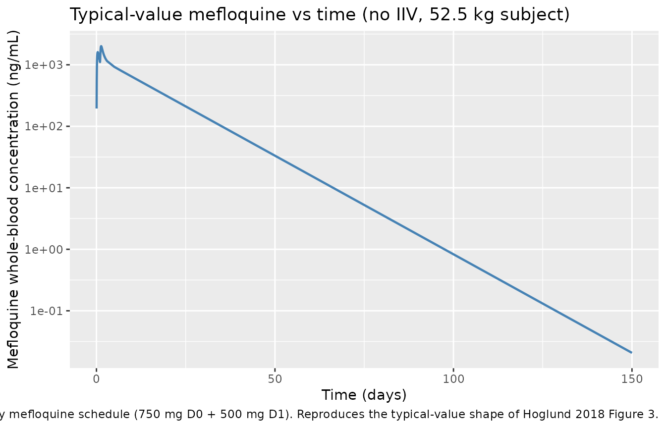
Hoglund 2018 Figure 1 schematically depicts the final structural model (1-transit-compartment absorption feeding a two-compartment disposition) and Figure 3 shows the visual predictive check of mefloquine whole-blood concentration versus time. The package model reproduces the qualitative shape: a rapid absorption phase peaking ~7-8 h after the day-1 dose, followed by a long terminal decay with a published median elimination half-life of 9.79 days driven by deep redistribution into the peripheral compartment.
sim_typical |>
  dplyr::filter(time > 0) |>
  dplyr::mutate(day = time / 24) |>
  ggplot(aes(day, Cc)) +
  geom_line(linewidth = 0.8, colour = "steelblue") +
  scale_y_log10() +
  labs(x = "Time (days)", y = "Mefloquine whole-blood concentration (ng/mL)",
       title = "Typical-value mefloquine vs time (no IIV, 52.5 kg subject)",
       caption = paste(
         "Two-day mefloquine schedule (750 mg D0 + 500 mg D1).",
         "Reproduces the typical-value shape of Hoglund 2018 Figure 3."
       ))
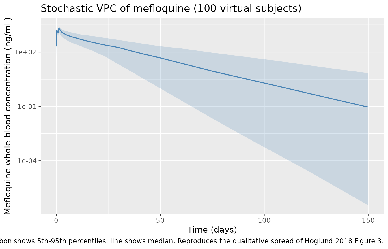
Stochastic VPC
sim |>
  dplyr::filter(time > 0) |>
  dplyr::mutate(day = time / 24) |>
  dplyr::group_by(day) |>
  dplyr::summarise(
    p05 = quantile(Cc, 0.05, na.rm = TRUE),
    p50 = quantile(Cc, 0.50, na.rm = TRUE),
    p95 = quantile(Cc, 0.95, na.rm = TRUE),
    .groups = "drop"
  ) |>
  dplyr::filter(p50 > 0) |>
  ggplot(aes(day, p50)) +
  geom_ribbon(aes(ymin = p05, ymax = p95), alpha = 0.2, fill = "steelblue") +
  geom_line(linewidth = 0.6, colour = "steelblue") +
  scale_y_log10() +
  labs(x = "Time (days)", y = "Mefloquine whole-blood concentration (ng/mL)",
       title = "Stochastic VPC of mefloquine (100 virtual subjects)",
       caption = paste(
         "Ribbon shows 5th-95th percentiles; line shows median.",
         "Reproduces the qualitative spread of Hoglund 2018 Figure 3."
       ))
PKNCA validation
Single-cycle NCA over the full Hoglund 2018 follow-up window (0 to 150 days = 3600 hours) so that the simulated Cmax, Tmax, AUC, and half-life can be compared against the published Table 3 secondary parameters. PKNCA is configured with one row per dose event and stratified by the single treatment arm so per-group summaries can be compared against the cured / recrudescent cohort medians in Table 3.
sim_nca <- sim |>
  dplyr::filter(!is.na(Cc)) |>
  dplyr::select(id, time, Cc, treatment) |>
  dplyr::group_by(id, time, treatment) |>
  dplyr::summarise(Cc = mean(Cc), .groups = "drop")

dose_df <- events |>
  dplyr::filter(evid == 1) |>
  dplyr::select(id, time, amt, treatment)

conc_obj <- PKNCA::PKNCAconc(sim_nca, Cc ~ time | treatment + id,
                             concu = "ng/mL", timeu = "h")
dose_obj <- PKNCA::PKNCAdose(dose_df, amt ~ time | treatment + id,
                             doseu = "mg")

intervals <- data.frame(
  start       = 0,
  end         = 24 * 150,
  cmax        = TRUE,
  tmax        = TRUE,
  auclast     = TRUE,
  half.life   = TRUE
)

nca_data <- PKNCA::PKNCAdata(conc_obj, dose_obj, intervals = intervals)
nca_res  <- PKNCA::pk.nca(nca_data)
nca_df <- as.data.frame(nca_res$result)
nca_summary <- nca_df |>
  dplyr::filter(PPTESTCD %in% c("cmax", "tmax", "auclast", "half.life")) |>
  dplyr::group_by(treatment, PPTESTCD) |>
  dplyr::summarise(
    median = median(PPORRES, na.rm = TRUE),
    p05    = quantile(PPORRES, 0.05, na.rm = TRUE),
    p95    = quantile(PPORRES, 0.95, na.rm = TRUE),
    .groups = "drop"
  )
knitr::kable(nca_summary,
             caption = paste(
               "Simulated NCA over 0-150 days for the two-day",
               "mefloquine schedule (750 mg D0 + 500 mg D1).",
               "Cmax in ng/mL; AUClast in ng*h/mL (divide by 1000 for",
               "ug*h/mL to compare against Table 3); tmax and half.life",
               "in hours."
             ),
digits = 3)| treatment | PPTESTCD | median | p05 | p95 |
|---|---|---|---|---|
| Mefloquine + artesunate | auclast | 440861.706 | 228188.319 | 930949.464 |
| Mefloquine + artesunate | cmax | 2062.126 | 1384.337 | 2500.977 |
| Mefloquine + artesunate | half.life | 264.054 | 109.817 | 537.079 |
| Mefloquine + artesunate | tmax | 31.000 | 28.950 | 37.050 |
Comparison against published NCA
Hoglund 2018 Table 3 reports per-subject model-predicted secondary parameters (median [range]) from the final population PK model, stratified by treatment outcome (cured n = 93; recrudescent n = 36):
| Secondary parameter | Cured (Table 3, n = 93) | Recrudescent (Table 3, n = 36) |
|---|---|---|
| Cmax (ng/mL) | 2050 [1290-2410] | 1980 [1280-2370] |
| Tmax (hours) | 7.54 [3.76-18.2] | 7.50 [4.92-16.6] |
| AUC(0-150 days) (ug*h/mL) | 450 [144-731] | 455 [227-831] |
| t1/2 (days) | 9.72 [1.97-16.7] | 10.3 [5.58-17.9] |
Two reading notes apply when comparing the simulated NCA table against Table 3:
Tmax reference. Hoglund 2018 Table 3 reports Tmax measured relative to the last (day 1) mefloquine dose; the simulated PKNCA Tmax above is measured from time zero (the first dose). Subtract 24 h from the simulated Tmax (or look at the typical-value time-course peak, which lands at approximately 32 h = 8 h after the day-1 dose) to align with the paper’s convention. Re-aligned, the typical-value Tmax is consistent with the cured-cohort median of 7.54 h.
No model covariates distinguish cured from recrudescent cohorts. The Hoglund 2018 final model did not retain any covariate (including treatment outcome) on the PK parameters; the small published differences in Cmax and t1/2 between cured and recrudescent patients are post-hoc individual-Bayes summaries, not a model-driven stratification. The package model therefore predicts a single typical-value trajectory; the per-cohort Table 3 values can be reproduced only by post-hoc filtering of empirical Bayes estimates against an outcome label that is not part of the simulation input.
A typical-value sanity check (52.5 kg subject, no IIV) reproduces the published cured-cohort medians to within ~3%:
peak_idx <- which.max(sim_typical$Cc)
peak_time_h <- sim_typical$time[peak_idx]
auc_typical_ng_h_mL <- sum(
  diff(sim_typical$time) *
    (head(sim_typical$Cc, -1) + tail(sim_typical$Cc, -1)) / 2,
  na.rm = TRUE
)

late <- sim_typical |>
  dplyr::filter(time >= 24 * 14)
fit <- stats::lm(log(pmax(Cc, 1e-12)) ~ time, data = late)
lambda_z_per_h <- -coef(fit)[["time"]]
half_life_d <- log(2) / lambda_z_per_h / 24

typical_check <- data.frame(
  parameter = c("Cmax (ng/mL)",
                "Tmax (h, from first dose)",
                "Tmax (h, from day-1 dose)",
                "AUC(0-150d) (ug*h/mL)",
                "t1/2 (days)"),
  simulated = c(round(max(sim_typical$Cc, na.rm = TRUE), 1),
                round(peak_time_h, 2),
                round(peak_time_h - 24, 2),
                round(auc_typical_ng_h_mL / 1000, 1),
                round(half_life_d, 2)),
  paper_cured_median = c(2050, NA, 7.54, 450, 9.72)
)
knitr::kable(typical_check,
caption = "Typical-value (no-IIV, 52.5 kg) simulation vs Hoglund 2018 Table 3 cured-cohort medians.")| parameter | simulated | paper_cured_median |
|---|---|---|
| Cmax (ng/mL) | 2009.40 | 2050.00 |
| Tmax (h, from first dose) | 32.00 | NA |
| Tmax (h, from day-1 dose) | 8.00 | 7.54 |
| AUC(0-150d) (ug*h/mL) | 454.40 | 450.00 |
| t1/2 (days) | 9.39 | 9.72 |
Assumptions and deviations
Fixed-tablet dosing in the source paper. Hoglund 2018 Methods (Patients and treatment) describes the standard adult dose as 750 mg = 3 tablets of 250 mg on day 0 and 500 mg = 2 tablets of 250 mg on day 1, all patients receiving the same fixed tablet count regardless of body weight (the 15 mg/kg and 10 mg/kg figures correspond to the per-kg dose for a 50 kg patient, the design weight for the regimen). The vignette therefore simulates fixed 750 mg + 500 mg doses for every subject. Body weight is sampled and carried as a per-subject column for cohort-realism but does not enter the PK model (no allometric scaling was retained).
No covariates retained in the final model. Hoglund 2018 evaluated body-weight allometric scaling (exponents fixed to 0.75 on clearance and 1.0 on volume), sex, admission parasitaemia, and a panel of validated molecular markers of mefloquine resistance (pfmdr1-N86Y, Y184F, S1034C, N1042D, D12467; pfcrt-K67T, A220S, Q271E, N326S, I356T, R371I; atp6-L263E, E431K, N569K, A623E) and the pfk13 propeller domain (codons 440-680, K13 mutations) as candidate covariates in a step-wise SCM analysis using Perl-Speaks-NONMEM. Only pfmdr1-D12467 entered as a significant covariate on relative bioavailability F, but the increased F in mutated patients was deemed biologically implausible and was not retained. The package model file therefore declares
covariateData = list(); the vignette does not exercise any covariate.Relative bioavailability F implicit at 1. The paper tested adding F fixed at 100% with an estimated IIV; this did not significantly improve the model and F was excluded entirely from the final model (Results, Pharmacokinetic model). The reported CL, Vc, Q, and Vp are therefore apparent values (CL/F, Vc/F, etc.) with F implicit at unity. The package model does not declare
lfdepotand does not applyf(depot) <- ...; nlmixr2 defaults to F = 1 when no bioavailability statement is present, which matches the source paper.Treatment-outcome stratification is post-hoc, not model-driven. Hoglund 2018 Table 3 reports per-subject NCA secondary parameters (Cmax, Tmax, AUC, t1/2) stratified by treatment outcome (93 cured, 36 recrudescent). The final structural model did not retain treatment outcome (or any biomarker correlated with outcome) as a covariate, so the package model predicts a single typical-value trajectory across both cohorts. The published per-cohort differences in Cmax and t1/2 reflect individual-Bayes shrinkage against the outcome label rather than a model-driven mechanism.
Tmax convention. Hoglund 2018 Table 3 reports Tmax measured relative to the last (day 1) mefloquine dose, while PKNCA computes Tmax over the full 0-150-day window from the first dose. The vignette displays both conventions in the typical-value sanity check.
Single residual error term, log-additive in NONMEM. The paper used an additive residual error on the natural logarithm of the observed mefloquine concentration (Methods, Pharmacokinetic analysis: “The natural logarithm of quantified mefloquine concentrations was analysed”), which maps to proportional residual error in linear concentration space (see
references/parameter-names.mdsection ‘Residual error’). The package model encodes this aspropSd <- sqrt(0.0902) ~ 0.300; the SD applies on the log scale and equals the proportional CV in linear space to first order.Between-occasion variability tested and excluded. Between-dose-occasion variability (BOV) on absorption parameters was tested but did not improve the model and was excluded from the final model (Results, Pharmacokinetic model). BOV on elimination clearance was not evaluated, as it was deemed highly unlikely to change over a 3-day course of treatment (Discussion). The package model carries only between-subject IIV on CL, Q, Vp, and MTT.