Abrocitinib concentration-QTc and heart rate (Wang 2022)
Source:vignettes/articles/Wang_2022_abrocitinib_QTc.Rmd
Wang_2022_abrocitinib_QTc.RmdModel and source
- Citation: Wang X, Gupta P, Malhotra BK, Farooqui SA, Le VH, Wojciechowski J, Mukherjee A, Nicholas T. Population Pharmacokinetic/Pharmacodynamic Modeling of the Effect of Abrocitinib on QT Intervals in Healthy Volunteers. Clin Pharmacol Drug Dev. 2022;11(9):1036-1045. doi:10.1002/cpdd.1111.
- Article: https://doi.org/10.1002/cpdd.1111
Wang et al. (2022) analysed the thorough-QT study of abrocitinib, a selective Janus kinase 1 inhibitor for moderate to severe atopic dermatitis. Healthy volunteers received single oral doses of abrocitinib 600 mg, placebo and moxifloxacin 400 mg in a randomized three-period crossover. Two prespecified linear mixed-effects models related the time-matched abrocitinib plasma concentration to the change from baseline in the Fridericia-corrected QT interval (DeltaQTcF) and in heart rate (DeltaHR). The package carries one file for each:
| Model file | Endpoint | Output | Source table |
|---|---|---|---|
Wang_2022_abrocitinib_QTcF |
DeltaQTcF (ms) | QTcF |
Table 1 |
Wang_2022_abrocitinib_HR |
DeltaHR (bpm) | d_hr |
Table 2 |
Both models share one structure (Wang 2022 Equations 1 and 3):
where TRT is 0 in the placebo period and 1 in the
abrocitinib period (ON_TREATMENT), C is the
abrocitinib plasma concentration (CP_ABROCITINIB_NGML, 0
for placebo), Y_ij0 is the period baseline
(QTC_BL or HR) and theta_k is a
free intercept shift for each nominal post-dose time other than the
first (NTIME, reference 0.25 h). Both random effects are
additive and correlated. The time-matched placebo-corrected effect used
for the regulatory assessment is therefore
Both are PD-only models: concentrations enter as data. To simulate
from a dose, this vignette drives them with the registry’s abrocitinib
population PK model, Wojciechowski_2022_abrocitinib
(Wojciechowski 2022, the population PK analysis cited by Wang 2022 for
the atopic-dermatitis Cmax).
Population
Thirty-six healthy adults (31 White, 3 Black, 2 other) were randomized; mean age 33.2 years (range 19-55), mean weight 80.2 kg (range 55.8-105.4), mean body mass index 24.7 kg/m^2 (Wang 2022 Results). The sex distribution is not reported. Mean baseline heart rate was 54.1-54.7 bpm and mean baseline QTcF 399.2-400.7 ms across the treatment groups. Triplicate ECGs were recorded at -1, -0.5 and 0 h before and at 0.25, 0.5, 1, 2, 3, 6, 12 and 24 h after each dose, with a PK sample at each post-dose ECG time. A total of 864 observations entered the concentration-QTc analysis; moxifloxacin data were used only to show assay sensitivity.
Source trace
| Element | Value | Source |
|---|---|---|
| Model structure (both endpoints) | linear mixed-effects, Eq. 1 / Eq. 3 | Methods |
QTcF e0 (theta0) |
-0.0062 ms | Table 1 |
QTcF slope (theta1) |
0.0026 ms/(ng/mL) | Table 1 |
QTcF e_on_treatment_e0 (theta2) |
0.3141 ms | Table 1 |
QTcF e_qtc_bl_e0 (theta3) |
-0.0577 ms/ms | Table 1 |
QTcF e_ntime0p5_e0 … e_ntime24_e0
(theta4-theta10) |
-2.678, -1.851, -3.152, -2.666, -7.052, -3.402, -5.103 ms | Table 1 |
| QTcF IIV SD intercept / slope / correlation | 3.315 ms / 0.0014 ms/(ng/mL) / -0.5294 | Table 1 |
| QTcF residual SD | 5.075 ms | Table 1 |
HR e0 (theta0) |
-0.669 bpm | Table 2 |
HR slope (theta1) |
0.0031 bpm/(ng/mL) | Table 2 |
HR e_on_treatment_e0 (theta2) |
-0.1979 bpm | Table 2 |
HR e_hr_bl_e0 (theta3) |
-0.1544 bpm/bpm | Table 2 |
HR e_ntime0p5_e0 … e_ntime24_e0
(theta4-theta10) |
0.0797, -0.299, -0.7794, -0.5218, 5.689, 4.274, 3.111 bpm | Table 2 |
| HR IIV SD intercept / slope / correlation | 1.594 bpm / 0.0016 bpm/(ng/mL) / -0.4389 | Table 2 |
| HR residual SD | 3.264 bpm | Table 2 |
| Baseline QTcF centering | 400 ms (assumed; groups 399.2-400.7) | Results |
| Baseline HR centering | 54.4 bpm (assumed; groups 54.1-54.7) | Results |
| Nominal ECG times | 0.25, 0.5, 1, 2, 3, 6, 12, 24 h | Methods |
| Validation targets: DeltaDeltaQTcF, DeltaDeltaHR at 1701 and 2156 ng/mL | 4.8 / 6.0 ms; 5.1 / 6.51 bpm | Table 3, Results |
Models
mod_qtcf <- readModelDb("Wang_2022_abrocitinib_QTcF")
mod_hr <- readModelDb("Wang_2022_abrocitinib_HR")

# Typical-value forms. `omega = NA` is also passed at each typical-value
# rxSolve() so that no etas are re-sampled from options retained by the
# compiled model.
mod_qtcf_typ <- rxode2::zeroRe(mod_qtcf)
mod_hr_typ <- rxode2::zeroRe(mod_hr)

ntime_levels <- c(0.25, 0.5, 1, 2, 3, 6, 12, 24)

# Event table for the PD-only models. There are no dosing records and no ODE
# states; every covariate is a column. The models are algebraic, so the rows
# can share one id with arbitrary increasing times.
pd_events <- function(conc, on_trt, ntime, qtc_bl = 400, hr_bl = 54.4) {
  n <- max(length(conc), length(on_trt), length(ntime))
  data.frame(
    id = 1L, time = seq_len(n), evid = 0L, amt = 0,
    CP_ABROCITINIB_NGML = rep_len(conc, n),
    ON_TREATMENT = rep_len(on_trt, n),
    NTIME = rep_len(ntime, n),
    QTC_BL = qtc_bl, HR = hr_bl
  )
}

solve_typ <- function(model, ev) {
  as.data.frame(rxode2::rxSolve(model, events = ev, omega = NA))
}
Structural checks
At zero concentration, in the placebo period and at the mean
baseline, each model must return exactly e0 at the 0.25 h
reference and e0 + theta_k at every other nominal time.
These are identities of the encoding, so they are asserted at machine
precision. They also confirm that the nominal-time binning selects the
intended level and that no random effect leaked into the typical-value
solve.
ev <- pd_events(conc = 0, on_trt = 0, ntime = ntime_levels)
chk_ntime <- data.frame(
  NTIME = ntime_levels,
  QTcF = solve_typ(mod_qtcf_typ, ev)$QTcF,
  d_hr = solve_typ(mod_hr_typ, ev)$d_hr
)
expected_qtcf <- -0.0062 +
  c(0, -2.678, -1.851, -3.152, -2.666, -7.052, -3.402, -5.103)
expected_hr <- -0.669 +
  c(0, 0.0797, -0.299, -0.7794, -0.5218, 5.689, 4.274, 3.111)
stopifnot(
  isTRUE(all.equal(chk_ntime$QTcF, expected_qtcf, tolerance = 1e-12)),
  isTRUE(all.equal(chk_ntime$d_hr, expected_hr, tolerance = 1e-12))
)

chk_ntime |>
  dplyr::rename(
    "Nominal time (h)" = NTIME,
    "Placebo DeltaQTcF (ms)" = QTcF,
    "Placebo DeltaHR (bpm)" = d_hr
  ) |>
knitr::kable(digits = 3, caption = "Typical placebo-period prediction at each nominal time (zero concentration, mean baseline).")| Nominal time (h) | Placebo DeltaQTcF (ms) | Placebo DeltaHR (bpm) |
|---|---|---|
| 0.25 | -0.006 | -0.669 |
| 0.50 | -2.684 | -0.589 |
| 1.00 | -1.857 | -0.968 |
| 2.00 | -3.158 | -1.448 |
| 3.00 | -2.672 | -1.191 |
| 6.00 | -7.058 | 5.020 |
| 12.00 | -3.408 | 3.605 |
| 24.00 | -5.109 | 2.442 |
The diurnal pattern of the nominal-time effects differs between the endpoints: QTcF is lowest 6 h after dosing, while heart rate rises by 4-6 bpm from 6 h onwards. These shifts are common to both periods and cancel in the placebo-corrected contrast.
Placebo-corrected effect at the supratherapeutic concentration (Table 3)
Wang 2022 Table 3 reports the model-predicted mean time-matched
placebo-corrected change from baseline at the concentration quoted for
healthy volunteers (1701 ng/mL) and at the supratherapeutic
concentration in atopic dermatitis (2156 ng/mL: the predicted 200 mg
once-daily steady-state Cmax of 1123 ng/mL times the 1.92-fold increase
under fluconazole). The model reproduces it as the difference between an
abrocitinib-period prediction at concentration C and a
placebo-period prediction at zero concentration, at the same nominal
time and baseline. The check is run at every nominal time and at
off-mean baselines, because all other terms must cancel.
ddelta <- function(model_typ, out, conc, ntime, qtc_bl = 400, hr_bl = 54.4) {
  act <- solve_typ(model_typ, pd_events(conc, 1, ntime, qtc_bl, hr_bl))[[out]]
  pbo <- solve_typ(model_typ, pd_events(0, 0, ntime, qtc_bl, hr_bl))[[out]]
  act - pbo
}

conc_tab3 <- c(1701, 2156)
tab3 <- data.frame(
  Population = c("Healthy volunteers", "Patients with AD"),
  conc = conc_tab3,
  qtcf_pub = c(4.8, 6.00),
  qtcf_sim = ddelta(mod_qtcf_typ, "QTcF", conc_tab3, ntime = 1),
  hr_pub = c(5.1, 6.51),
  hr_sim = ddelta(mod_hr_typ, "d_hr", conc_tab3, ntime = 1)
) |>
  dplyr::mutate(
    qtcf_pct = 100 * (qtcf_sim - qtcf_pub) / qtcf_pub,
    hr_pct = 100 * (hr_sim - hr_pub) / hr_pub
  )

# The contrast must not depend on the nominal time or the baseline.
grid <- expand.grid(ntime = ntime_levels, qtc_bl = c(380, 420), hr_bl = c(45, 65))
spread <- vapply(seq_len(nrow(grid)), function(i) {
  q <- ddelta(mod_qtcf_typ, "QTcF", 2156, grid$ntime[i], grid$qtc_bl[i], grid$hr_bl[i])
  h <- ddelta(mod_hr_typ, "d_hr", 2156, grid$ntime[i], grid$qtc_bl[i], grid$hr_bl[i])
  max(abs(q - tab3$qtcf_sim[2]), abs(h - tab3$hr_sim[2]))
}, numeric(1))

stopifnot(
  max(spread) < 1e-10,
  # Exact identity with the closed form theta2 + theta1 * C
  isTRUE(all.equal(tab3$qtcf_sim, 0.3141 + 0.0026 * conc_tab3, tolerance = 1e-12)),
  isTRUE(all.equal(tab3$hr_sim, -0.1979 + 0.0031 * conc_tab3, tolerance = 1e-12)),
  # Against the published means; the residual gap is the 2-significant-figure
  # rounding of the printed slopes (see below).
  all(abs(tab3$qtcf_pct) < 3),
  all(abs(tab3$hr_pct) < 3)
)

tab3 |>
  dplyr::select(Population, conc, qtcf_pub, qtcf_sim, qtcf_pct, hr_pub, hr_sim, hr_pct) |>
  dplyr::rename(
    "Concentration (ng/mL)" = conc,
    "DeltaDeltaQTcF published (ms)" = qtcf_pub,
    "DeltaDeltaQTcF model (ms)" = qtcf_sim,
    "QTcF % diff" = qtcf_pct,
    "DeltaDeltaHR published (bpm)" = hr_pub,
    "DeltaDeltaHR model (bpm)" = hr_sim,
    "HR % diff" = hr_pct
  ) |>
knitr::kable(digits = 2, caption = "Replicates Table 3 of Wang 2022 (mean placebo-corrected effects).")| Population | Concentration (ng/mL) | DeltaDeltaQTcF published (ms) | DeltaDeltaQTcF model (ms) | QTcF % diff | DeltaDeltaHR published (bpm) | DeltaDeltaHR model (bpm) | HR % diff |
|---|---|---|---|---|---|---|---|
| Healthy volunteers | 1701 | 4.8 | 4.74 | -1.32 | 5.10 | 5.08 | -0.49 |
| Patients with AD | 2156 | 6.0 | 5.92 | -1.34 | 6.51 | 6.49 | -0.37 |
The model reproduces the published means within 1.3% (QTcF) and 0.5%
(HR). The gap is the rounding of the printed slopes: solving Table 3 for
the QTcF slope, (6.00 - 0.3141) / 2156 and
(4.8 - 0.3141) / 1701 both give 0.00264 ms/(ng/mL), which
Table 1 prints as 0.0026. The model keeps the printed value. The 90%
confidence intervals of Table 3 cannot be reproduced because they depend
on the sampling covariance of theta1 and theta2, which is not
reported.
conc_grid <- seq(0, 4500, by = 50)
curve_df <- dplyr::bind_rows(
  data.frame(endpoint = "DeltaDeltaQTcF (ms)", conc = conc_grid,
             value = ddelta(mod_qtcf_typ, "QTcF", conc_grid, ntime = 1)),
  data.frame(endpoint = "DeltaDeltaHR (bpm)", conc = conc_grid,
             value = ddelta(mod_hr_typ, "d_hr", conc_grid, ntime = 1))
)
ggplot(curve_df, aes(conc, value)) +
  geom_line() +
  geom_vline(xintercept = 2156, linetype = "dashed", colour = "steelblue") +
  geom_hline(yintercept = 10, linetype = "dotted", colour = "firebrick") +
  facet_wrap(~endpoint) +
  labs(x = "Abrocitinib concentration (ng/mL)", y = "Placebo-corrected change from baseline") +
  theme_bw()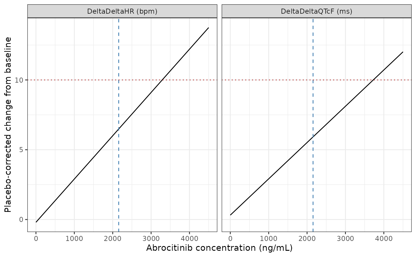
Typical placebo-corrected effect across the studied concentration range. Replicates the mean lines of Figures 4 and 5 of Wang 2022; the dashed vertical line is the 2156 ng/mL supratherapeutic concentration and the dotted horizontal line the 10 ms / 10 bpm threshold.
Driving the models from a dose
The PD models need an abrocitinib concentration at each ECG time.
Here they come from Wojciechowski_2022_abrocitinib for a
single 600 mg dose in healthy adults. The formulation of the thorough-QT
tablets is not stated; the commercial (phase III) tablet is assumed.
Covariates follow the reported demographics: weight drawn from a normal
distribution with the reported mean and truncated at the reported range,
2 of 36 subjects (5.6%) of other race, and all subjects male because the
sex split is not reported.
n_sub <- 120
pk_mod <- readModelDb("Wojciechowski_2022_abrocitinib")

set.seed(20221109)
wt <- pmin(pmax(rnorm(n_sub, 80.2, 12), 55.8), 105.4)
cov_df <- data.frame(
  id = seq_len(n_sub), WT = wt, SEXF = 0, RACE_ASIAN = 0,
  RACE_OTHER = as.integer(seq_len(n_sub) %% 18 == 0),
  ADOLESCENT = 0, DIS_PSORIASIS = 0, DIS_ATOPIC_DERMATITIS = 0,
  HEPIMP_MILD = 0, HEPIMP_MOD = 0,
  CONMED_RIFAMPICIN = 0, CONMED_FLUCONAZOLE = 0, CONMED_FLUVOXAMINE = 0,
  FED_HIGHFAT = 0, FORM_ABROCITINIB_SUSP = 0, FORM_ABROCITINIB_TAB_PH2B = 0,
  FORM_ABROCITINIB_TAB_PH3 = 1, MULTI_DOSE = 0,
  DOSE_ABROCITINIB_MG = 600, DOSE_ABROCITINIB_MGD = 600,
  STUDY_B7451005 = 0, STUDY_B7451006 = 0, STUDY_B7451012 = 0,
  STUDY_B7451043 = 0
)

# Dense grid for NCA plus the nominal ECG times; each dose is a depot record
# and a rate = -1 central record (see the Wojciechowski 2022 vignette).
obs_times <- sort(unique(c(0, seq(0.25, 4, by = 0.25), 5:12, 16, 20, 24, ntime_levels)))
pk_events <- dplyr::bind_rows(
  data.frame(time = 0, amt = 600, evid = 1L, cmt = "depot", rate = 0),
  data.frame(time = 0, amt = 600, evid = 1L, cmt = "central", rate = -1),
  data.frame(time = obs_times, amt = 0, evid = 0L, cmt = "central", rate = 0)
)
pk_events <- merge(cov_df, pk_events, by = NULL) |>
  dplyr::select(id, time, amt, evid, cmt, rate, dplyr::everything()) |>
  dplyr::arrange(id, time, dplyr::desc(evid))

pk_sim <- as.data.frame(rxode2::rxSolve(pk_mod, events = pk_events, returnType = "data.frame")) |>
  dplyr::select(id, time, Cc) |>
  dplyr::mutate(treatment = "abrocitinib 600 mg")
PKNCA on the driving concentrations
conc_obj <- PKNCA::PKNCAconc(
  pk_sim |> dplyr::filter(!is.na(Cc)),
  Cc ~ time | treatment + id
)
dose_obj <- PKNCA::PKNCAdose(
  data.frame(id = seq_len(n_sub), time = 0, amt = 600, treatment = "abrocitinib 600 mg"),
  amt ~ time | treatment + id
)
intervals <- data.frame(start = 0, end = 24, cmax = TRUE, tmax = TRUE, auclast = TRUE)
nca_res <- PKNCA::pk.nca(PKNCA::PKNCAdata(conc_obj, dose_obj, intervals = intervals))

nca_summary <- as.data.frame(nca_res$result) |>
  dplyr::filter(PPTESTCD %in% c("cmax", "tmax", "auclast")) |>
  dplyr::group_by(PPTESTCD) |>
  dplyr::summarise(
    geomean = exp(mean(log(PPORRES))),
    median = stats::median(PPORRES),
    p05 = stats::quantile(PPORRES, 0.05),
    p95 = stats::quantile(PPORRES, 0.95),
    .groups = "drop"
  )
knitr::kable(nca_summary, digits = 2, caption = "NCA of the simulated 600 mg single-dose profiles (0-24 h).")| PPTESTCD | geomean | median | p05 | p95 |
|---|---|---|---|---|
| auclast | 11293.75 | 12382.29 | 5016.06 | 25438.61 |
| cmax | 1764.33 | 1792.55 | 853.00 | 3387.75 |
| tmax | 2.78 | 2.75 | 2.75 | 2.75 |
cmp <- nlmixr2lib::ncaComparisonTable(
  simulated = nca_res,
  reference = data.frame(treatment = "abrocitinib 600 mg", cmax = 1701),
  by = "treatment",
  units = c(cmax = "ng/mL"),
  tolerance_pct = 20
)
knitr::kable(cmp, caption = "Simulated median Cmax against the 1701 ng/mL healthy-volunteer concentration of Wang 2022 Table 3.")| NCA parameter | treatment | Reference | Simulated | % diff |
|---|---|---|---|---|
| Cmax (ng/mL) | abrocitinib 600 mg | 1700 | 1790 | +5.4% |
Wang 2022 does not report NCA for this study. The exposure information it gives is the 1701 ng/mL quoted for healthy volunteers in Table 3, a maximum observed concentration above 4000 ng/mL, and the mean concentration-time profile of Figure 3c, which peaks at the 3 h sample. The simulated Tmax of 2.75 h is the end of the zero-order absorption arm that the PK model applies to doses above 121 mg, which is why it is the same in every subject. The comparison is a plausibility check of the PK driver, not a test of the QTc models: the upstream PK model was fitted to other studies, and its formulation and sex inputs here are assumptions.
# Approximate means read from Wang 2022 Figure 3c (ng/mL).
fig3c_obs <- data.frame(
  time = ntime_levels,
  conc = c(240, 810, 1140, 1510, 1950, 1030, 270, 70)
)
pk_sim |>
  dplyr::filter(time %in% ntime_levels) |>
  dplyr::distinct(id, time, .keep_all = TRUE) |>
  dplyr::group_by(time) |>
  dplyr::summarise(
    mean = mean(Cc),
    lo = mean - stats::qt(0.95, dplyr::n() - 1) * stats::sd(Cc) / sqrt(dplyr::n()),
    hi = mean + stats::qt(0.95, dplyr::n() - 1) * stats::sd(Cc) / sqrt(dplyr::n()),
    .groups = "drop"
  ) |>
  ggplot(aes(time, mean)) +
  geom_line() +
  geom_errorbar(aes(ymin = lo, ymax = hi), width = 0.3) +
  geom_point(data = fig3c_obs, aes(time, conc), colour = "firebrick", size = 2) +
  labs(x = "Time after dose (h)", y = "Abrocitinib concentration (ng/mL)") +
  theme_bw()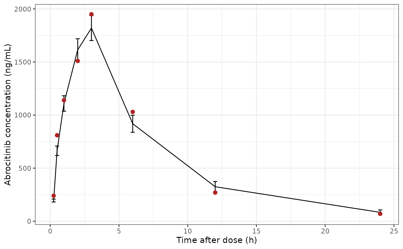
Simulated mean (90% CI) concentration at the nominal ECG times against the observed means of Figure 3c of Wang 2022 (red; read from the figure by the maintainers, approximate).
Simulated crossover
Each simulated subject contributes an abrocitinib period (concentration from the PK simulation at each nominal ECG time) and a placebo period (concentration 0), with one set of random effects per subject as in the source model. Baseline QTcF and HR are drawn from normal distributions centred on the reported means; their spreads (SD 15 ms and 7 bpm) are assumptions because the paper reports only the means.
pd_cov <- data.frame(
  id = seq_len(n_sub),
  QTC_BL = rnorm(n_sub, 400, 15),
  HR = rnorm(n_sub, 54.4, 7)
)
conc_at_ecg <- pk_sim |>
  dplyr::filter(time %in% ntime_levels) |>
  dplyr::distinct(id, time, .keep_all = TRUE) |>
  dplyr::transmute(id, NTIME = time, CP_ABROCITINIB_NGML = Cc)

pd_ev <- dplyr::bind_rows(
  conc_at_ecg |> dplyr::mutate(ON_TREATMENT = 1, period = "abrocitinib", time = NTIME),
  conc_at_ecg |> dplyr::mutate(ON_TREATMENT = 0, period = "placebo", time = 100 + NTIME,
                               CP_ABROCITINIB_NGML = 0)
) |>
  dplyr::left_join(pd_cov, by = "id") |>
  dplyr::mutate(evid = 0L, amt = 0) |>
  dplyr::select(id, time, evid, amt, dplyr::everything()) |>
  dplyr::arrange(id, time)

sim_qtcf <- as.data.frame(rxode2::rxSolve(mod_qtcf, events = pd_ev, keep = c("period", "NTIME", "CP_ABROCITINIB_NGML")))
sim_hr <- as.data.frame(rxode2::rxSolve(mod_hr, events = pd_ev, keep = c("period", "NTIME", "CP_ABROCITINIB_NGML")))

pd_long <- dplyr::bind_rows(
  sim_qtcf |> dplyr::transmute(id, period, NTIME, conc = CP_ABROCITINIB_NGML,
                               endpoint = "QTcF (ms)", value = sim),
  sim_hr |> dplyr::transmute(id, period, NTIME, conc = CP_ABROCITINIB_NGML,
                             endpoint = "HR (bpm)", value = sim)
)

# Time-matched placebo correction within subject
pd_dd <- pd_long |>
  tidyr::pivot_wider(id_cols = c(id, NTIME, endpoint), names_from = period, values_from = c(value, conc)) |>
  dplyr::mutate(ddelta = value_abrocitinib - value_placebo, conc = conc_abrocitinib)
pd_long |>
  dplyr::filter(period == "abrocitinib") |>
  ggplot(aes(conc, value)) +
  geom_point(alpha = 0.25, size = 0.8) +
  geom_smooth(method = "lm", formula = y ~ x, colour = "firebrick", linetype = "dashed") +
  facet_wrap(~endpoint, scales = "free_y") +
  labs(x = "Abrocitinib concentration (ng/mL)", y = "Change from baseline") +
  theme_bw()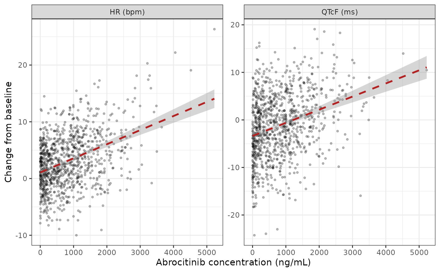
Simulated change from baseline against abrocitinib concentration in the abrocitinib period with a linear fit. Replicates the layout of Figure 1 of Wang 2022.
fig3_df <- dplyr::bind_rows(
  pd_dd |> dplyr::transmute(NTIME, panel = paste0("DeltaDelta", endpoint), y = ddelta),
  conc_at_ecg |> dplyr::transmute(NTIME, panel = "Concentration (ng/mL)", y = CP_ABROCITINIB_NGML)
) |>
  dplyr::group_by(panel, NTIME) |>
  dplyr::summarise(
    mean = mean(y),
    lo = mean - stats::qt(0.95, dplyr::n() - 1) * stats::sd(y) / sqrt(dplyr::n()),
    hi = mean + stats::qt(0.95, dplyr::n() - 1) * stats::sd(y) / sqrt(dplyr::n()),
    .groups = "drop"
  )
ggplot(fig3_df, aes(NTIME, mean)) +
  geom_line() +
  geom_point() +
  geom_errorbar(aes(ymin = lo, ymax = hi), width = 0.3) +
  facet_wrap(~panel, ncol = 1, scales = "free_y") +
  labs(x = "Nominal time after dose (h)", y = NULL) +
  theme_bw()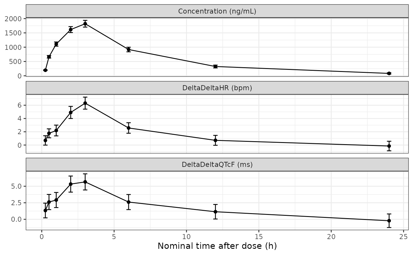
Mean (90% CI) simulated placebo-corrected change from baseline and mean concentration over time. Replicates Figure 3 of Wang 2022: the effect peaks with the concentration, with no delay.
Regressing the simulated placebo-corrected effects on concentration should recover the model slopes, because the nominal-time and baseline terms cancel within subject. The regression slope is compared with the model slope with a tolerance of 30%: several standard errors wide for 120 subjects (realised differences are about 3-10%), while a mis-transcribed slope or a unit error moves it by far more.
fit_slopes <- pd_dd |>
  dplyr::group_by(endpoint) |>
  dplyr::summarise(
    slope_hat = unname(stats::coef(stats::lm(ddelta ~ conc))[2]),
    .groups = "drop"
  ) |>
  dplyr::mutate(
    slope_model = ifelse(endpoint == "QTcF (ms)", 0.0026, 0.0031),
    pct_diff = 100 * (slope_hat - slope_model) / slope_model
  )
stopifnot(all(abs(fit_slopes$pct_diff) < 30))
fit_slopes |>
  dplyr::rename(
    "Endpoint" = endpoint,
    "Regression slope (per ng/mL)" = slope_hat,
    "Model slope (per ng/mL)" = slope_model,
    "% diff" = pct_diff
  ) |>
knitr::kable(digits = 5, caption = "Slope of simulated placebo-corrected effect on concentration.")| Endpoint | Regression slope (per ng/mL) | Model slope (per ng/mL) | % diff |
|---|---|---|---|
| HR (bpm) | 0.00319 | 0.0031 | 2.79460 |
| QTcF (ms) | 0.00285 | 0.0026 | 9.64054 |
Assumptions and deviations
- Centering constants. The models centre baseline QTcF and HR on “the overall mean of all the baseline values”, which the paper does not print. The rounded values 400 ms and 54.4 bpm sit inside the reported ranges of treatment-group means (399.2-400.7 ms and 54.1-54.7 bpm); the resulting error in any prediction is below 0.05 ms or 0.05 bpm.
-
Nominal-time reference. The reference level is the
first post-dose time, 0.25 h, as stated for theta0 (“placebo, at the
first postdose sampling time”).
NTIMEis binned to the nearest scheduled level inside the model, so a value between grid points is assigned to the closest one. -
Treatment indicator in a crossover.
ON_TREATMENTis constant within a period and changes between periods. Each subject has one intercept and one slope random effect across periods, as in the source model. - Rounded slopes. Table 1 prints the QTcF slope as 0.0026; Table 3 implies 0.00264. The printed value is kept, which places the model 1.3% below the published DeltaDeltaQTcF means.
- Correction-factor model not packaged. Equation 2 (a log-log QT-RR model used to derive a study-specific correction) reports only its estimated exponent, 0.3375; Fridericia (0.333) was used for the primary analysis.
-
Upstream PK. The concentration driver in this
vignette is the separately published
Wojciechowski_2022_abrocitinibmodel with an assumed commercial tablet formulation and all-male cohort; the QTc and HR models themselves were fitted to observed concentrations. - Figure 3c means. The observed mean concentrations overlaid on the PK driver were read from Figure 3c by eye and are approximate; they are shown for comparison only and are not used by any assertion.
- Baseline spreads. The SDs of baseline QTcF and HR used in the simulated cohort are assumptions.
- Metabolites. The active metabolites M1 and M2 were not measured or modelled; the models describe parent abrocitinib only.