Tacrolimus (Chen 2022b)
Source:vignettes/articles/Chen_2022b_tacrolimus.Rmd
Chen_2022b_tacrolimus.RmdModel and source
- Citation: Chen X, Wang D, Zheng F, Zhai X, Xu H, Li Z. Population pharmacokinetics and initial dose optimization of tacrolimus in children with severe combined immunodeficiency undergoing hematopoietic stem cell transplantation. Front Pharmacol. 2022;13:869939. doi:10.3389/fphar.2022.869939
- Description: One-compartment population PK model with first-order absorption and first-order elimination for oral tacrolimus whole-blood concentrations in Chinese children with severe combined immunodeficiency (SCID) undergoing haematopoietic stem cell transplantation (Chen 2022). The absorption rate constant ka is fixed at 4.48 1/h from earlier paediatric tacrolimus models. Apparent oral clearance CL/F is allometrically scaled by body weight (fixed exponent 0.75, reference 70 kg) and apparent volume V/F scales linearly with body weight (fixed exponent 1). Exponential IIV on CL/F and V/F; combined proportional-plus-additive residual error.
- Article: https://doi.org/10.3389/fphar.2022.869939 (open access, PMC9354257)
Chen et al. (2022) fitted a one-compartment model with first-order absorption in NONMEM (FOCE-I) to routine therapeutic-drug-monitoring tacrolimus concentrations from children with severe combined immunodeficiency (SCID) undergoing haematopoietic stem cell transplantation (HSCT), and used Monte Carlo simulation to recommend an initial dose for children weighing 5-20 kg. The final model (Results, Eqs. 6-7) is
- CL/F (L/h) = 13.1 x (WT/70)^0.75
- V/F (L) = 10900 x (WT/70)
- Ka = 4.48 1/h (fixed)
with exponential IIV on CL/F and V/F and a combined proportional-plus-additive residual error.
Population
Eighteen Chinese children with SCID (14 boys, 4 girls) undergoing HSCT at the Children’s Hospital of Fudan University between February 2016 and April 2021 contributed 130 tacrolimus whole-blood concentrations (mean 7.2 per patient). Table 1: age median 0.70 (range 0.33-3.01) years, weight median 7.50 (4.20-12.60) kg, albumin median 33.2 g/L, haematocrit median 26.6%. Co-medications: caspofungin 9, ethambutol 10, glucocorticoids 17, isoniazid 14, micafungin 9, mycophenolic acid 6, omeprazole 13, vancomycin 10; none was retained as a covariate. Whole-blood tacrolimus was measured by the Emit 2000 assay (2.0-30 ng/mL). Doses and sampling times are not tabulated.
Source trace
| Element | Value | Source |
|---|---|---|
| Structure: 1-compartment, first-order absorption and elimination | – | Methods, Population pharmacokinetic model |
lka |
4.48 1/h (fixed) | Table 2; Methods (Yang et al. 2015; Wang et al. 2019) |
lcl |
13.1 L/h | Table 2; Eq. 6 |
lvc |
10900 L | Table 2 (109 in units of 10^2 L); Eq. 7 |
e_wt_cl |
0.75 (fixed), reference 70 kg | Methods Eq. 3; Eq. 6 |
e_wt_vc |
1 (fixed), reference 70 kg | Methods Eq. 3; Eq. 7 |
Exponential IIV Wi = T(U) * exp(eta)
|
– | Methods Eq. 1 |
etalcl |
0.451^2 = 0.203401 | Table 2 (omega CL/F = 0.451, read as SD; see Assumptions) |
etalvc |
0.592^2 = 0.350464 | Table 2 (omega V/F = 0.592, read as SD) |
Residual error Mi = Ni * (1 + eps1) + eps2
|
– | Methods Eq. 2 |
propSd |
0.257 | Table 2 (sigma 1, proportional) |
addSd |
1.265 ng/mL | Table 2 (sigma 2, additive) |
Typical CL/F per kg (Figure 3A)
The Abstract and Results state that the typical CL/F falls from 0.36 to 0.26 L/h/kg between 5 and 20 kg, and Figure 3A plots the curve. Both follow from Eq. 6 alone.
mod <- readModelDb("Chen_2022b_tacrolimus")
mod_typ <- rxode2::zeroRe(mod)
#> ℹ parameter labels from comments will be replaced by 'label()'

ev_cl <- tibble(id = 1:16, WT = 5:20, time = 1, amt = 0, evid = 0L, cmt = "central")
cl_typ <- rxode2::rxSolve(mod_typ, events = ev_cl, keep = "WT") |>
  as.data.frame() |>
  mutate(cl_per_kg = cl / WT)
#> ℹ omega/sigma items treated as zero: 'etalcl', 'etalvc'
#> Warning: multi-subject simulation without without 'omega'

cl_typ |>
  filter(WT %in% c(5, 10, 15, 20)) |>
  select(WT, cl, cl_per_kg) |>
  dplyr::rename("Weight (kg)" = WT, "CL/F (L/h)" = cl, "CL/F (L/h/kg)" = cl_per_kg) |>
knitr::kable(digits = 3)| Weight (kg) | CL/F (L/h) | CL/F (L/h/kg) |
|---|---|---|
| 5 | 1.810 | 0.362 |
| 10 | 3.044 | 0.304 |
| 15 | 4.126 | 0.275 |
| 20 | 5.119 | 0.256 |
# The text quotes the end points to two decimal places.
stopifnot(
  round(cl_typ$cl_per_kg[cl_typ$WT == 5], 2) == 0.36,
  round(cl_typ$cl_per_kg[cl_typ$WT == 20], 2) == 0.26
)
ggplot(cl_typ, aes(WT, cl_per_kg)) +
  geom_line(colour = "darkgreen") +
  geom_point() +
  scale_x_continuous(limits = c(0, 25)) +
  labs(x = "Body weight (kg)", y = "CL/F (L/h/kg)")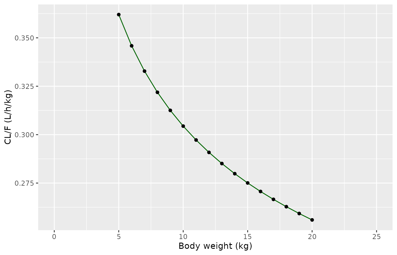
Typical CL/F per kg by body weight. Replicates Figure 3A of Chen 2022.
Target attainment (Figures 3B-E and 4)
Chen 2022 simulated 1,000 virtual patients at each of four body weights (5, 10, 15 and 20 kg) and eight daily doses (0.1-0.8 mg/kg/day, given as two equal doses), and plotted the probability that the tacrolimus concentration falls in the 5-20 ng/mL target range (Figure 4). The simulation time is not stated; the pre-dose trough on day 4 (72 h, just before the seventh twice-daily dose) reproduces Figure 4 and is used here (see Assumptions).
The model is linear in dose, so each weight is simulated once at 1
mg/kg/day and the concentration rescaled for each dose. Each weight has
196 virtual subjects whose CL/F and V/F random effects sit on a 14 x 14
grid of evenly spaced quantiles of their normal distributions rather
than being drawn at random, which makes the target-attainment
percentages deterministic. Residual error is not added (the model’s
Cc is the individual prediction); the Assumptions section
explains why.
tau <- 12
ndose <- 15
weights <- c(5, 10, 15, 20)
nq <- 14
om <- sqrt(diag(rxode2::rxode(mod)$omega))
#> ℹ parameter labels from comments will be replaced by 'label()'
zq <- qnorm(ppoints(nq))

subj <- tidyr::expand_grid(WT = weights, kc = seq_len(nq), kv = seq_len(nq)) |>
  mutate(id = row_number(), etalcl = om[["etalcl"]] * zq[kc], etalvc = om[["etalvc"]] * zq[kv])

# Observe just before each dose from the 2nd to the 15th (troughs after
# 1-14 doses); the 1e-6 h offset keeps each sample ahead of its dose.
t_trough <- seq(tau, by = tau, length.out = ndose - 1) - 1e-6
ev_pta <- bind_rows(
  tidyr::expand_grid(id = subj$id, time = seq(0, by = tau, length.out = ndose)) |>
    mutate(evid = 1L, cmt = "depot"),
  tidyr::expand_grid(id = subj$id, time = t_trough) |>
    mutate(evid = 0L, cmt = "central")
) |>
  left_join(select(subj, id, WT), by = "id") |>
  mutate(amt = ifelse(evid == 1L, 1 * WT / 2, 0)) |> # 1 mg/kg/day split in two
  arrange(id, time, desc(evid))

# The etas are supplied per subject, so rxode2 draws none itself.
sim_pta <- suppressWarnings(rxode2::rxSolve(
  mod,
  events = ev_pta, params = select(subj, id, etalcl, etalvc),
  keep = "WT"
)) |>
  as.data.frame() |>
  mutate(n_doses = round(time / tau))
#> ℹ parameter labels from comments will be replaced by 'label()'

# round() makes each level the same double as the literal in fig4 below
dose_levels <- round(seq(0.1, 0.8, by = 0.1), 1)
pta_of <- function(sim, with_ruv = FALSE) {
  tidyr::expand_grid(sim |> select(id, WT, n_doses, Cc), dose = dose_levels) |>
    mutate(
      conc = Cc * dose,
      sd_ruv = sqrt((conc * 0.257)^2 + 1.265^2),
      p_in = if (with_ruv) {
        pnorm(20, conc, sd_ruv) - pnorm(5, conc, sd_ruv)
      } else {
        as.numeric(conc >= 5 & conc <= 20)
      }
    ) |>
    group_by(WT, n_doses, dose) |>
    summarise(pta = 100 * mean(p_in), .groups = "drop")
}
pta_all <- pta_of(sim_pta)
pta <- filter(pta_all, n_doses == 6)
sim_pta |>
  filter(n_doses == 6) |>
  tidyr::expand_grid(dose = dose_levels) |>
  mutate(conc = Cc * dose, WT = paste(WT, "kg")) |>
  ggplot(aes(factor(dose), conc, colour = factor(dose))) +
  geom_jitter(width = 0.3, height = 0, size = 0.4, show.legend = FALSE) +
  geom_hline(yintercept = c(5, 20), linetype = "dashed", colour = "red") +
  facet_wrap(~WT) +
  labs(x = "Daily dose (mg/kg/day)", y = "Tacrolimus (ng/mL)")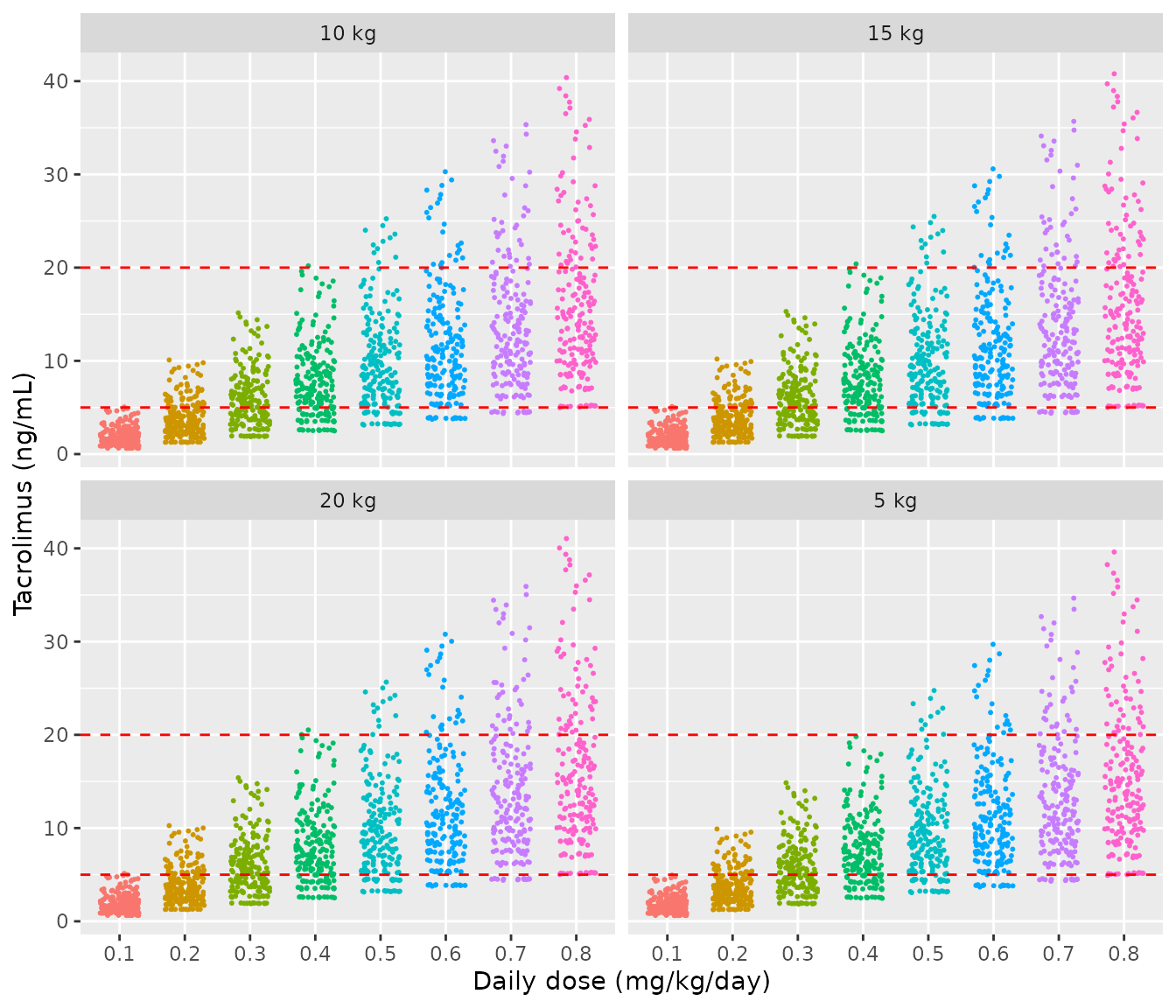
Simulated pre-dose concentrations on day 4 by daily dose for each body weight; dashed lines mark the 5-20 ng/mL target. Replicates Figures 3B-E of Chen 2022 (the published panels are random draws; these are the quantile-grid subjects).
# Figure 4 of Chen 2022, digitised by the maintainers (gridlines every 10%)
fig4 <- tibble::tribble(
  ~dose, ~p5, ~p10, ~p15, ~p20,
  0.1, 1.8, 2.0, 2.1, 2.2,
  0.2, 24.0, 25.6, 26.1, 26.6,
  0.3, 51.6, 53.0, 53.6, 54.2,
  0.4, 71.0, 71.5, 71.8, 72.0,
  0.5, 79.6, 79.8, 79.2, 79.0,
  0.6, 83.0, 81.7, 81.2, 80.7,
  0.7, 78.7, 77.8, 76.8, 76.4,
  0.8, 72.8, 71.2, 70.7, 70.2
) |>
  tidyr::pivot_longer(starts_with("p"), names_to = "WT", values_to = "fig4_pta") |>
  mutate(WT = as.numeric(sub("p", "", WT)))

ggplot(pta, aes(WT, pta, colour = factor(dose))) +
  geom_line() +
  geom_point(data = fig4, aes(y = fig4_pta)) +
  scale_x_continuous(limits = c(0, 25)) +
  labs(x = "Body weight (kg)", y = "P(5-20 ng/mL) (%)", colour = "Dose (mg/kg/day)")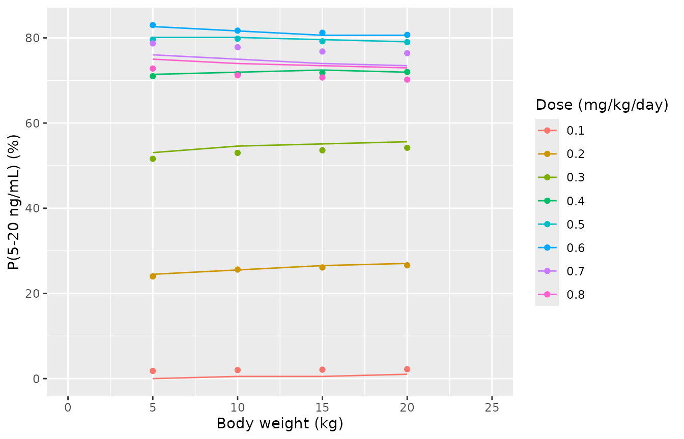
Simulated probability of a day-4 pre-dose concentration in 5-20 ng/mL by body weight and daily dose (lines); points are Figure 4 of Chen 2022 digitised by the maintainers. Replicates Figure 4 of Chen 2022.
cmp4 <- inner_join(fig4, pta, by = c("dose", "WT")) |>
  mutate(diff = pta - fig4_pta)
cmp4 |>
  group_by(WT) |>
  summarise(median_abs_diff = median(abs(diff)), max_abs_diff = max(abs(diff)), .groups = "drop") |>
  dplyr::rename(
    "Weight (kg)" = WT, "Median |difference| (percentage points)" = median_abs_diff,
    "Max |difference| (percentage points)" = max_abs_diff
  ) |>
knitr::kable(digits = 1)| Weight (kg) | Median |difference| (percentage points) | Max |difference| (percentage points) |
|---|---|---|
| 5 | 1.0 | 2.7 |
| 10 | 1.0 | 2.8 |
| 15 | 1.1 | 2.8 |
| 20 | 0.8 | 2.9 |
best <- pta |>
  group_by(WT) |>
  slice_max(pta, n = 1, with_ties = FALSE) |>
  ungroup()

# The replication is deterministic (quantile-placed etas, no residual error),
# so these bounds do not depend on the random-number stream. The published
# curves carry their own Monte Carlo noise (1,000 subjects per cell) and a
# digitisation error of about 1 point.
stopifnot(
  nrow(cmp4) == 32,
  median(abs(cmp4$diff)) < 3,
  quantile(abs(cmp4$diff), 0.9) < 6,
  # The recommended 0.6 mg/kg/day attains the target most often at every weight.
  all(abs(best$dose - 0.6) < 1e-9)
)
The same replication under the alternative readings of Table 2 – omega as a variance rather than an SD, residual error included in the simulated concentrations – and at other simulation times matches Figure 4 less well:
# Variance reading: re-solve with each eta on sqrt(omega) instead of omega.
sim_var <- suppressWarnings(rxode2::rxSolve(
  mod,
  events = ev_pta,
  params = select(subj, id, etalcl, etalvc) |>
    mutate(
      etalcl = etalcl / om[["etalcl"]] * sqrt(om[["etalcl"]]),
      etalvc = etalvc / om[["etalvc"]] * sqrt(om[["etalvc"]])
    ),
  keep = "WT"
)) |>
  as.data.frame() |>
  mutate(n_doses = round(time / tau))

rmse_by_time <- function(p) {
  inner_join(fig4, p, by = c("dose", "WT")) |>
    group_by(n_doses) |>
    summarise(rmse = sqrt(mean((pta - fig4_pta)^2)), .groups = "drop")
}
scan <- bind_rows(
  rmse_by_time(pta_all) |> mutate(reading = "omega as SD, no residual error (used)"),
  rmse_by_time(pta_of(sim_pta, TRUE)) |> mutate(reading = "omega as SD, with residual error"),
  rmse_by_time(pta_of(sim_var)) |> mutate(reading = "omega as variance, no residual error"),
  rmse_by_time(pta_of(sim_var, TRUE)) |> mutate(reading = "omega as variance, with residual error")
)
scan |>
  filter(n_doses %in% c(4, 5, 6, 7, 8, 10, 14)) |>
  mutate(n_doses = paste0("after ", n_doses, " doses (", n_doses * tau, " h)")) |>
  tidyr::pivot_wider(names_from = n_doses, values_from = rmse) |>
  dplyr::rename("Reading of Table 2" = reading) |>
knitr::kable(digits = 1, caption = "RMSE against Figure 4 (percentage points) by reading and pre-dose sampling time.")| Reading of Table 2 | after 4 doses (48 h) | after 5 doses (60 h) | after 6 doses (72 h) | after 7 doses (84 h) | after 8 doses (96 h) | after 10 doses (120 h) | after 14 doses (168 h) |
|---|---|---|---|---|---|---|---|
| omega as SD, no residual error (used) | 15.4 | 6.6 | 1.6 | 6.2 | 11.7 | 22.3 | 37.0 |
| omega as SD, with residual error | 15.3 | 7.9 | 4.9 | 8.0 | 12.5 | 21.0 | 34.3 |
| omega as variance, no residual error | 16.3 | 10.8 | 8.4 | 10.7 | 14.5 | 20.7 | 32.3 |
| omega as variance, with residual error | 17.7 | 13.0 | 11.6 | 12.9 | 15.4 | 21.1 | 31.1 |
best_each <- scan |>
  group_by(reading) |>
  summarise(n_doses = n_doses[which.min(rmse)], rmse = min(rmse), .groups = "drop")
used <- best_each$reading == "omega as SD, no residual error (used)"
stopifnot(
  # The reading used is best at the day-4 trough ...
  best_each$n_doses[used] == 6,
  # ... and beats every alternative, at its own best time, by a clear margin.
  all(best_each$rmse[used] * 2.5 < best_each$rmse[!used])
)
PKNCA validation
The paper reports no NCA. As a structural check, a typical-value
subject (zeroRe()) at each of the four simulation weights
receives a single 0.3 mg/kg dose (one half of the recommended 0.6
mg/kg/day); PKNCA computes AUC0-inf and the terminal half-life, which
must equal the closed forms Dose / (CL/F) and
log(2) * (V/F) / (CL/F). Sampling runs to 3,000 h because
the half-life is about 300-420 h at these weights.
nca_subj <- tibble(id = seq_along(weights), WT = weights, treatment = paste(weights, "kg")) |>
  mutate(amt = 0.3 * WT)
t_grid <- c(0, 0.25, 0.5, 0.75, 1, 1.5, 2, 3, 4, 6, 8, 12, 24, 48, 96, 168, 336, 500, 750, 1000, 1500, 2000, 2500, 3000)
ev_nca <- bind_rows(
  nca_subj |> mutate(time = 0, evid = 1L, cmt = "depot"),
  tidyr::expand_grid(id = nca_subj$id, time = t_grid) |>
    left_join(select(nca_subj, id, WT, treatment), by = "id") |>
    mutate(amt = 0, evid = 0L, cmt = "central")
) |>
  arrange(id, time, desc(evid))

sim_nca <- rxode2::rxSolve(mod_typ, events = ev_nca, keep = "treatment") |>
  as.data.frame()
#> ℹ omega/sigma items treated as zero: 'etalcl', 'etalvc'
#> Warning: multi-subject simulation without without 'omega'

conc <- sim_nca |>
  filter(!is.na(Cc)) |>
  select(id, time, Cc, treatment)
doses_nca <- nca_subj |>
  mutate(time = 0) |>
  select(id, time, amt, treatment)

o_conc <- PKNCAconc(conc, Cc ~ time | treatment + id)
o_dose <- PKNCAdose(doses_nca, amt ~ time | treatment + id)
intervals <- data.frame(start = 0, end = Inf, cmax = TRUE, tmax = TRUE, aucinf.obs = TRUE, half.life = TRUE)
nca_res <- pk.nca(PKNCAdata(o_conc, o_dose, intervals = intervals))

pars <- sim_nca |>
  distinct(treatment, cl, vc)
nca_wide <- as.data.frame(nca_res) |>
  filter(PPTESTCD %in% c("cmax", "tmax", "aucinf.obs", "half.life")) |>
  select(treatment, PPTESTCD, PPORRES) |>
  tidyr::pivot_wider(names_from = PPTESTCD, values_from = PPORRES) |>
  left_join(nca_subj, by = "treatment") |>
  left_join(pars, by = "treatment") |>
  mutate(auc_closed = 1000 * amt / cl, thalf_closed = log(2) * vc / cl)

nca_wide |>
  arrange(WT) |>
  select(treatment, amt, cmax, tmax, aucinf.obs, auc_closed, half.life, thalf_closed) |>
  dplyr::rename(
    "Weight" = treatment, "Dose (mg)" = amt, "Cmax (ng/mL)" = cmax, "Tmax (h)" = tmax,
    "AUC0-inf (PKNCA, ng*h/mL)" = aucinf.obs, "Dose/(CL/F) (ng*h/mL)" = auc_closed,
    "t1/2 (PKNCA, h)" = half.life, "log(2) V/CL (h)" = thalf_closed
  ) |>
knitr::kable(digits = 2, caption = "Typical-value single-dose NCA at 0.3 mg/kg.")| Weight | Dose (mg) | Cmax (ng/mL) | Tmax (h) | AUC0-inf (PKNCA, ng*h/mL) | Dose/(CL/F) (ng*h/mL) | t1/2 (PKNCA, h) | log(2) V/CL (h) |
|---|---|---|---|---|---|---|---|
| 5 kg | 1.5 | 1.92 | 1.5 | 828.69 | 828.74 | 298.16 | 298.16 |
| 10 kg | 3.0 | 1.92 | 2.0 | 985.49 | 985.54 | 354.57 | 354.57 |
| 15 kg | 4.5 | 1.92 | 2.0 | 1090.63 | 1090.68 | 392.40 | 392.40 |
| 20 kg | 6.0 | 1.92 | 2.0 | 1171.96 | 1172.01 | 421.66 | 421.66 |
Assumptions and deviations
-
IIV and residual-error scale. Table 2 reports
“omega CL/F = 0.451”, “omega V/F = 0.592”, “sigma 1 = 0.257”
(proportional) and “sigma 2 = 1.265” (additive) without stating whether
they are variances or standard deviations. Replicating Figure 4 settles
it: with the omegas as SDs and no residual error, the deterministic
replication above reproduces all 32 digitised points with a
root-mean-square error of about 1.6 percentage points; reading the
omegas as variances (SDs 0.67 and 0.77) makes that error at least five
times larger at any sampling time (table above). The SD reading is used,
and sigma 1 and sigma 2 are read on the same scale as omega in the same
table (proportional SD 25.7%, additive SD 1.265 ng/mL). This is the
scale settled the same way for earlier models by the same group
(
Chen_2020b_tacrolimus,Wang_2019b_tacrolimus). - Residual error in Figure 4. Adding the residual error to the simulated concentrations widens the distribution and triples the error against Figure 4 (table above), so the published simulations appear to be of individual predictions. The replication above excludes residual error accordingly; the model file keeps it for simulating observations.
- Simulation time for Figure 4. Not stated. The pre-dose trough on day 4 (72 h, after six twice-daily doses) reproduces the curves, including the peak at 0.6 mg/kg/day and the fall-off at 0.7-0.8 mg/kg/day; earlier and later troughs do not (table above). Steady state is far off at that time: the typical half-life is about 300-420 h at 5-20 kg.
- Very large V/F. Table 2 prints V/F as 109 in units of 10^2 L and Eq. 7 as 10900 L at 70 kg, i.e. about 156 L/kg, which gives the long half-life above. Both printings agree and the Figure 4 replication depends on this magnitude (at 72 h the concentration is close to cumulative dose / V/F), so the value is used as printed.
- Fixed ka. 4.48 1/h is taken from earlier paediatric tacrolimus models (Yang et al. 2015; Wang et al. 2019 in the paper’s references) and was not estimated.
- Reference weight. The 70 kg reference lies far outside the observed 4.2-12.6 kg range, so 13.1 L/h and 10900 L are adult-equivalent extrapolations.
- Small cohort. The model was fitted to 18 children; the bootstrap intervals in Table 2 are wide (e.g. omega CL/F 0.003-0.748), and the authors call for a larger cohort to confirm the results.