Model and source
- Citation: Nie X, Gao X, Gao J, Heng T, Zhang Y, Sun Y, Feng Z, Jia L, Wang M. Population pharmacokinetics of nalbuphine in patients undergoing general anesthesia surgery. Front Pharmacol. 2023;14:1130287. doi:10.3389/fphar.2023.1130287.
- Article (open access): https://doi.org/10.3389/fphar.2023.1130287
- Supplement: none. Frontiers in Pharmacology published no Supporting Information for this article, and none is required – every final parameter estimate is printed in Table 4 and the final-model equations are printed in-line in Results section 3.2.
Nie 2023 is a single-centre prospective population PK analysis of nalbuphine given as a single intravenous injection for induction of general anaesthesia. Nalbuphine is a semi-synthetic opioid that agonises the kappa receptor while partially antagonising the mu receptor, which is why it is used at induction: it provides analgesia with a ceiling on respiratory depression.
The distinguishing feature of the model is its single
retained covariate. The authors screened the usual demographic
and hepatic panel and found that neither body weight nor age entered the
final model; what survived forward inclusion and backward elimination
was an intra-operative quantity – the hourly net fluid volume infused
(HNF), entering intercompartmental clearance Q as a power
function. That negative result is the paper’s main clinical message:
because weight does not scale the PK, a fixed 12 mg dose and a
weight-based 0.2 mg/kg dose give exposures that differ by less than 6%,
and the fixed regimen carries the lower variability.
mod <- readModelDb("Nie_2023_nalbuphine")
mod
#> function() {
#>   description <- paste(
#>     "Two-compartment IV population PK model of nalbuphine in adult patients undergoing general",
#>     "anaesthesia surgery (Nie 2023; 47 Chinese adults aged 21-78 years and 48-86 kg receiving a",
#>     "single 15 mg nalbuphine intravenous injection over 2-3 min for induction of anaesthesia,",
#>     "split into a 27-patient / 353-sample model-building set and a 20-patient / 100-sample",
#>     "external-validation set). Disposition is parameterized as CL, central volume V1,",
#>     "intercompartmental clearance Q and peripheral volume V2, with dosing directly into the",
#>     "central compartment (intravenous injection; no absorption phase). The single covariate",
#>     "retained by forward-inclusion / backward-elimination is the hourly net fluid volume infused",
#>     "during surgery, which enters Q as a power function; the authors attribute the effect to",
#>     "intra-operative changes in hepatic blood flow, nalbuphine having a hepatic extraction ratio",
#>     "of 0.5-0.7. Between-subject variability is exponential on all four disposition parameters",
#>     "and residual error is combined additive plus proportional.",
#>     sep = " "
#>   )
#>   reference <- paste(
#>     "Nie X, Gao X, Gao J, Heng T, Zhang Y, Sun Y, Feng Z, Jia L, Wang M.",
#>     "Population pharmacokinetics of nalbuphine in patients undergoing general anesthesia surgery.",
#>     "Front Pharmacol. 2023;14:1130287.",
#>     "doi:10.3389/fphar.2023.1130287.",
#>     sep = " "
#>   )
#>   vignette <- "Nie_2023_nalbuphine"
#>
#>   # Nie 2023 reports plasma nalbuphine concentrations in ng/mL (LLOQ 0.1 ng/mL,
#>   # calibration range 0.1-500 ng/mL; Methods 2.2) and volumes in L, so the
#>   # amount unit that makes `central / vc` come out in ng/mL directly is the
#>   # microgram (ug/L == ng/mL). Doses are therefore expressed in ug: the 15 mg
#>   # clinical induction dose is 15000 ug and the 12 mg simulated fixed dose is
#>   # 12000 ug. Encoding the dose in mg instead would force the paper's printed
#>   # additive residual error (2.88 ng/mL) to be rewritten as 0.00288 mg/L, i.e.
#>   # a unit conversion applied to a published value, which this library avoids.
#>   units <- list(time = "h", dosing = "ug", concentration = "ng/mL")
#>
#>   compartmentData <- list(
#>     central = list(
#>       analyte = "nalbuphine",
#>       units = "ug",
#>       specimen = "plasma",
#>       verified = TRUE
#>     ),
#>     peripheral1 = list(
#>       analyte = "nalbuphine",
#>       units = "ug",
#>       specimen = "tissue",
#>       verified = TRUE
#>     )
#>   )
#>
#>   covariateData <- list(
#>     PFA_NET_RATE = list(
#>       description = "Hourly net fluid volume infused during surgery",
#>       units = "mL/h",
#>       type = "continuous",
#>       reference_category = NULL,
#>       notes = paste(
#>         "Source column HNF. Nie 2023 Table 1 footnote defines it as",
#>         "HNF = (FVI + BVI - UVO) / OT, where FVI is the fluid volume infused, BVI the blood",
#>         "volume infused and UVO the urine volume output during surgery, and OT the operation",
#>         "time -- i.e. a net intra-operative fluid balance expressed as a rate. Time-fixed per",
#>         "subject (one scalar per operation). Model-building cohort 617.96 +/- 247.61 mL/h",
#>         "(median 563.56, range 234.26-1202.25); external-validation cohort 634.19 +/- 178.94",
#>         "mL/h (median 610.42, range 314.29-1047.24). The final model normalizes by 617.96 mL/h",
#>         "-- the model-building cohort MEAN, not the median. Nie 2023 Eq. 2 states the generic",
#>         "power form as theta1 * (cov_i / cov_median)^theta2, but the printed final-model",
#>         "equation (Results section 3.2) is Q = 245 * (HNF/617.96)^-0.58 and 617.96 is the mean",
#>         "from Table 1. The printed equation is used here per the standing rule that a printed",
#>         "equation outranks conflicting prose. Enters Q only; the negative exponent means a",
#>         "higher net intra-operative fluid load gives a LOWER intercompartmental clearance.",
#>         "One subject was dropped from the external-validation set for a missing HNF value",
#>         "(Results 3.1).",
#>         sep = " "
#>       ),
#>       source_name = "HNF"
#>     )
#>   )
#>
#>   # Screened during covariate model building (Nie 2023 Table 3) but NOT retained
#>   # in the final model, so they are documented rather than declared: none of
#>   # them is referenced in model(). ALT is the notable case -- it entered the
#>   # full model on CL (dOFV -7.39, p < 0.01) but was removed in backward
#>   # elimination because its dOFV of 7.40 did not exceed the 7.88 retention
#>   # criterion (Table 3 model 22, "> 0.005"), which the Discussion attributes to
#>   # the small sample and to most hepatic patients having ALT within 3x the
#>   # upper limit of normal.
#>   covariatesDataExcluded <- list(
#>     ALT = list(
#>       description = "Alanine aminotransferase",
#>       units = "U/L",
#>       type = "continuous",
#>       notes = paste(
#>         "Tested on CL as an exponential function (Nie 2023 Table 3 models 2 and 20, functional",
#>         "expression 'a' = Eq. 1 linear per the table footnote key). Entered the full model",
#>         "(OFV 2158.168 -> 2150.776 alone; 2148.529 -> 2141.133 on top of HNF-on-Q) but was",
#>         "eliminated in the backward step (dOFV 7.40 < 7.88). No point estimate is printed for",
#>         "the ALT coefficient anywhere in the paper, so the effect cannot be reconstructed.",
#>         sep = " "
#>       )
#>     ),
#>     GGT = list(
#>       description = "Gamma-glutamyltransferase",
#>       units = "U/L",
#>       type = "continuous",
#>       notes = "Tested on CL (Table 3 model 3, dOFV -4.90) and on V2 (model 13, dOFV -7.02); not retained. No coefficient printed."
#>     ),
#>     HR = list(
#>       description = "Heart rate",
#>       units = "beats/min",
#>       type = "continuous",
#>       notes = "Tested on V1 (Table 3 model 5, dOFV -7.06) and on Q (model 8, dOFV -5.88); not retained. No coefficient printed."
#>     ),
#>     WT = list(
#>       description = "Total body weight",
#>       units = "kg",
#>       type = "continuous",
#>       notes = paste(
#>         "Tested on V2 only (Table 3 model 12, dOFV -4.07) and not retained; no allometric",
#>         "scaling appears anywhere in the final model. This is the paper's central dosing",
#>         "finding -- because body weight does not enter the PK, a fixed 12 mg dose and a",
#>         "0.2 mg/kg weight-based dose differ only by the cohort mean dose (bias < 6% at every",
#>         "sampled time, Table 6), and the fixed regimen carries the lower exposure variability",
#>         "(Figure 8). Weight is still needed as a COHORT attribute to simulate the weight-based",
#>         "arm, but it is not a model covariate.",
#>         sep = " "
#>       )
#>     ),
#>     UA = list(
#>       description = "Uric acid",
#>       units = "umol/L",
#>       type = "continuous",
#>       notes = "Tested on V2 (Table 3 model 14, dOFV -5.37); not retained. No coefficient printed."
#>     ),
#>     DDIMER = list(
#>       description = "Plasma D-dimer",
#>       units = "mg/L",
#>       type = "continuous",
#>       notes = "Tested on V2 (Table 3 model 15, dOFV -4.79); not retained. No coefficient printed."
#>     ),
#>     SMOKE = list(
#>       description = "Current-smoker indicator",
#>       units = "(binary)",
#>       type = "binary",
#>       notes = "Tested on V2 (Table 3 model 19, dOFV -3.94); not retained. No coefficient printed. Table 1: 11/27 (40.7%) in the model-building cohort."
#>     )
#>   )
#>
#>   population <- list(
#>     species = "human",
#>     n_subjects = 47L,
#>     n_studies = 1L,
#>     age_range = "21-78 years overall; model-building cohort 53.85 +/- 16.63 years (median 58, range 21-76), external-validation cohort 52.5 +/- 13.56 (median 54.5, range 27-78)",
#>     age_median = "58 years (model-building cohort, Table 1)",
#>     weight_range = "48-86 kg overall; model-building cohort 63.32 +/- 9.3 kg (median 62, range 48-82), external-validation cohort 62.25 +/- 9.67 (median 59.5, range 50.8-86)",
#>     weight_median = "62 kg (model-building cohort, Table 1)",
#>     height_range = "Model-building cohort 163.96 +/- 6.87 cm (median 165, range 153-175)",
#>     sex_female_pct = 55.6,
#>     race_ethnicity = "Not reported; single-centre Chinese cohort",
#>     disease_state = "Adults scheduled for elective surgery under general anaesthesia. Liver resection 14.8%, cholecystectomy 12.8%, pancreatic resection 36.2%, other surgery 36.2%; 29.8% laparoscopic and 70.2% open. Model-building cohort: tumour 77.8%, hepatobiliary disease 55.6%, hypertension 25.9%, Child-Turcotte-Pugh class B 18.5% (the remainder class A).",
#>     dose_range = "Single nalbuphine 15 mg intravenous injection over 2-3 min at induction (0.24 +/- 0.04 mg/kg), followed by midazolam 0.05 mg/kg, sufentanil 0.2 ug/kg, etomidate 0.03 mg/kg and cisatracurium 0.2 mg/kg; anaesthesia maintained with sevoflurane and remifentanil",
#>     regions = "China (Shijiazhuang; the Fourth Hospital of Hebei Medical University, single centre, 2021)",
#>     hepatic_function = "55.6% of the model-building cohort had hepatobiliary disease; 18.5% were Child-Turcotte-Pugh class B and the rest class A. Excluded: known or suspected cardiopulmonary, renal or metabolic disease.",
#>     renal_function = "Creatinine clearance (Cockcroft-Gault) 111.19 +/- 27.38 mL/min in the model-building cohort (median 105.14, range 53.4-160.98)",
#>     co_medication = "Midazolam, sufentanil, etomidate, cisatracurium, sevoflurane and remifentanil, all part of the anaesthetic protocol. Nie 2023 Discussion notes as a limitation that nalbuphine, midazolam, sufentanil and sevoflurane are all CYP3A4 substrates and that the study design could not resolve any interaction between them.",
#>     notes = "Baseline demographics per Nie 2023 Table 1. 458 concentrations were drawn from 48 patients; one subject (5 samples) was dropped for a missing HNF value, leaving 27 patients / 353 samples for model building (intensive sampling: pre-dose and 3, 5, 10, 15, 30, 45 min and 1, 1.5, 2, 3, 4, 5, 6, 12 h) and 20 patients / 100 samples for external validation (sparse sampling: pre-dose, during intubation, and 1, 3, 10 min after intubation). Every post-dose sample was above the 0.1 ng/mL LLOQ and none was flagged as an outlier."
#>   )
#>
#>   ini({
#>     # Structural parameters, Nie 2023 Table 4 "Final model / Estimates" column.
#>     # The paper prints the final-model equations directly (Results 3.2):
#>     #   CL (L/h) = 32.9
#>     #   V1 (L)   = 32.5
#>     #   Q  (L/h) = 245 * (HNF/617.96)^-0.58
#>     #   V2 (L)   = 83.5
#>     # (Table 4's legend gives the units; the printed "Q (L)" line is a typo for
#>     # L/h, since Table 4 and the Discussion both state Q in L/h.)
#>     # All fixed-effect RSEs are < 30% and every estimate falls inside the
#>     # 2.5th-97.5th percentile of the 1000-sample bootstrap (984 successful
#>     # minimizations), so no parameter is poorly identified.
#>     lcl <- log(32.9); label("Clearance CL (L/h)")                                  # Nie 2023 Table 4 final model CL = 32.9 L/h (RSE 5.47%; bootstrap median 32.8, 95% CI 29.46-36.54)
#>     lvc <- log(32.5); label("Central volume V1 (L)")                               # Nie 2023 Table 4 final model V1 = 32.5 L (RSE 10.25%; bootstrap median 31.9, 95% CI 25.90-38.10)
#>     lq  <- log(245);  label("Intercompartmental clearance Q at PFA_NET_RATE = 617.96 mL/h (L/h)")  # Nie 2023 Table 4 final model Q = 245 L/h (RSE 13.99%; bootstrap median 247, 95% CI 216.63-297.38)
#>     lvp <- log(83.5); label("Peripheral volume V2 (L)")                            # Nie 2023 Table 4 final model V2 = 83.5 L (RSE 7.94%; bootstrap median 84.6, 95% CI 70.70-97.34)
#>
#>     # Power-function exponent for the hourly net fluid volume infused on Q,
#>     # normalized to 617.96 mL/h. Applied in model() as
#>     # (PFA_NET_RATE / 617.96)^e_pfa_net_rate_q, matching the printed equation.
#>     e_pfa_net_rate_q <- -0.58; label("Power exponent of hourly net fluid volume infused on Q (unitless)")  # Nie 2023 Table 4 final model "HNF on Q" = -0.58 (RSE 14.11%; bootstrap median -0.557, 95% CI -0.802 to -0.084)
#>
#>     # Between-subject variability, exponential on every disposition parameter
#>     # (Methods 2.3.1: "BSV ... was assumed to be log-normally distributed and
#>     # was applied by exponential model").
#>     #
#>     # Table 4 labels the BSV column "%CV", but the values printed there are the
#>     # NONMEM omega standard deviations x 100, not the exact log-normal CV. The
#>     # tell is the residual-error block of the SAME column: the final-model
#>     # proportional error prints as 0.139 while the basic model's (Table 2)
#>     # prints as 13.7 under the identical "%CV" header -- the software is
#>     # printing the raw parameter and the header is a mislabel. Reading the BSV
#>     # entries the same way, omega_CL = 0.277, omega_V1 = 0.401, omega_Q = 0.179
#>     # and omega_V2 = 0.408, so the variances below are those values squared.
#>     # This reading is corroborated by Results 3.2, which subtracts the numbers
#>     # arithmetically -- "a decrease in BSV from 35.5% to 17.9%, indicating that
#>     # 17.6% of BSV in Q was explained by HNF" (35.5 - 17.9 = 17.6) -- which is
#>     # only meaningful on the omega scale.
#>     etalcl ~ 0.076729  # Nie 2023 Table 4 final model omega CL = 27.7 -> 0.277^2 = 0.076729 (RSE 12.26%, shrinkage 4.30%)
#>     etalvc ~ 0.160801  # Nie 2023 Table 4 final model omega V1 = 40.1 -> 0.401^2 = 0.160801 (RSE 22.92%, shrinkage 13.10%)
#>     etalq  ~ 0.032041  # Nie 2023 Table 4 final model omega Q  = 17.9 -> 0.179^2 = 0.032041 (RSE 42.65%, shrinkage 30.72%; down from 35.5 in the basic model once HNF entered Q)
#>     etalvp ~ 0.166464  # Nie 2023 Table 4 final model omega V2 = 40.8 -> 0.408^2 = 0.166464 (RSE 13.84%, shrinkage 3.18%)
#>
#>     # Residual unexplained variability: combined proportional + additive
#>     # (Methods 2.3.1 tested proportional, additive and combined; Results 3.2
#>     # selected the combination).
#>     propSd <- 0.139; label("Proportional residual error (fraction)")  # Nie 2023 Table 4 final model proportional error = 0.139 (RSE 8.02%, shrinkage 12.79%; the basic model prints the same quantity as 13.7 in Table 2)
#>     addSd  <- 2.88;  label("Additive residual error (ng/mL)")         # Nie 2023 Table 4 final model additive error = 2.88 ng/mL (RSE 19.81%; bootstrap median 2.9035, 95% CI 1.88-4.72)
#>   })
#>
#>   model({
#>     # Individual disposition parameters. Only Q carries a covariate; CL, V1 and
#>     # V2 are covariate-free in the final model (weight and age were both
#>     # screened and rejected -- see covariatesDataExcluded and the Discussion).
#>     cl <- exp(lcl + etalcl)
#>     vc <- exp(lvc + etalvc)
#>     vp <- exp(lvp + etalvp)
#>
#>     # Q = 245 * (HNF/617.96)^-0.58 (Nie 2023 Results 3.2 printed equation).
#>     # 617.96 mL/h is the model-building cohort MEAN hourly net fluid volume
#>     # infused (Table 1), so exp(lq) is Q for a patient at that mean fluid load.
#>     q <- exp(lq + etalq) * (PFA_NET_RATE / 617.96)^e_pfa_net_rate_q
#>
#>     # Two-compartment IV disposition micro-constants.
#>     kel <- cl / vc
#>     k12 <- q / vc
#>     k21 <- q / vp
#>
#>     # Nalbuphine is given as an intravenous injection at induction, so doses
#>     # enter `central` directly from the event table; there is no depot and no
#>     # bioavailability term.
#>     d/dt(central)     <- -kel * central - k12 * central + k21 * peripheral1
#>     d/dt(peripheral1) <-                  k12 * central - k21 * peripheral1
#>
#>     # Plasma nalbuphine concentration in ng/mL (amounts in ug, volumes in L).
#>     Cc <- central / vc
#>     Cc ~ add(addSd) + prop(propSd)
#>   })
#> }
#> <environment: 0x56005531dab8>
Population
The analysis enrolled 47 adults scheduled for elective surgery at the Fourth Hospital of Hebei Medical University (Shijiazhuang, China) during 2021. All received nalbuphine 15 mg intravenously over 2-3 min at induction, followed by midazolam, sufentanil, etomidate and cisatracurium; anaesthesia was maintained with sevoflurane and remifentanil.
458 concentrations were drawn from 48 patients. One subject (5 samples) was dropped for a missing HNF value, leaving 27 patients / 353 samples in the model-building set (intensive sampling: pre-dose and 3, 5, 10, 15, 30, 45 min and 1, 1.5, 2, 3, 4, 5, 6, 12 h) and 20 patients / 100 samples in the external-validation set (sparse sampling: pre-dose, during intubation, and 1, 3, 10 min after intubation). Every post-dose sample was above the 0.1 ng/mL LLOQ and none was flagged as an outlier.
Model-building cohort baseline characteristics (Table 1), reported as mean +/- SD (median, range):
| Characteristic | Model-building (n = 27) |
|---|---|
| Age (years) | 53.85 +/- 16.63 (58, 21-76) |
| Total body weight (kg) | 63.32 +/- 9.3 (62, 48-82) |
| Height (cm) | 163.96 +/- 6.87 (165, 153-175) |
| Dose (mg/kg) | 0.24 +/- 0.04 (0.24, 0.18-0.31) |
| Hourly net fluid volume infused (mL/h) | 617.96 +/- 247.61 (563.56, 234.26-1202.25) |
| Operation duration (h) | 4.31 +/- 1.9 (4, 0.83-8.33) |
| Creatinine clearance (mL/min) | 111.19 +/- 27.38 (105.14, 53.4-160.98) |
| Alanine aminotransferase (U/L) | 58.86 +/- 69.62 (23.6, 6-260.9) |
| Female | 15 (55.6%) |
| Tumour | 21 (77.8%) |
| Hepatobiliary disease | 15 (55.6%) |
| Child-Turcotte-Pugh class B | 5 (18.5%) |
Across the whole cohort, liver resection accounted for 14.8%, cholecystectomy 12.8%, pancreatic resection 36.2% and other surgery 36.2%; 29.8% of procedures were laparoscopic and 70.2% open.
Source trace
Every value in the model file, with the location in Nie 2023 it came from.
| Model element | Value | Source |
|---|---|---|
| Structural model | 2-compartment IV | Results 3.2 (“a two-compartment model … decreased AIC by 519.209” vs 1-compartment) |
lcl |
CL = 32.9 L/h | Table 4 final model; Results 3.2 printed equation
CL (L/h) = 32.9
|
lvc |
V1 = 32.5 L | Table 4 final model; Results 3.2 printed equation
V1 (L) = 32.5
|
lq |
Q = 245 L/h | Table 4 final model; Results 3.2 printed equation |
lvp |
V2 = 83.5 L | Table 4 final model; Results 3.2 printed equation
V2 (L) = 83.5
|
e_pfa_net_rate_q |
-0.58 | Table 4 final model, row “HNF on Q” |
| Q covariate form | 245 * (HNF/617.96)^-0.58 |
Results 3.2 printed equation |
| HNF normalizing constant | 617.96 mL/h | Table 1, model-building cohort mean HNF |
| HNF definition | (FVI + BVI - UVO) / OT |
Table 1 footnote |
etalcl |
omega CL = 0.277 | Table 4 final model, omega CL = 27.7 |
etalvc |
omega V1 = 0.401 | Table 4 final model, omega V1 = 40.1 |
etalq |
omega Q = 0.179 | Table 4 final model, omega Q = 17.9 |
etalvp |
omega V2 = 0.408 | Table 4 final model, omega V2 = 40.8 |
| IIV form | exponential (log-normal) | Methods 2.3.1 |
propSd |
0.139 | Table 4 final model, proportional error |
addSd |
2.88 ng/mL | Table 4 final model, additive error |
| Residual form | combined additive + proportional | Methods 2.3.1; Results 3.2 |
| Dosing route | IV injection into central
|
Methods 2.1 (15 mg over 2-3 min at induction) |
| Concentration units | ng/mL | Methods 2.2 (LLOQ 0.1 ng/mL, range 0.1-500 ng/mL) |
Reading Table 4’s “%CV” column
Table 4 heads the random-effects column “%CV”, but the numbers
printed under it are the NONMEM omega standard deviations multiplied by
100 rather than exact log-normal coefficients of variation. The tell is
the residual-error block of the same column: the final model
prints the proportional error as 0.139 while the basic
model (Table 2) prints the identical quantity as 13.7. The
software is printing the raw parameter and the header is a mislabel.
Reading the BSV rows the same way gives omega = 0.277, 0.401, 0.179 and
0.408, which is what the model file encodes (as variances, i.e. those
values squared).
This reading is corroborated by Results 3.2, which subtracts the numbers arithmetically – “a decrease in BSV from 35.5% to 17.9%, indicating that 17.6% of BSV in Q was explained by HNF” (35.5 - 17.9 = 17.6). That subtraction is only meaningful on the omega scale.
Structural verification against a closed form
A two-compartment model dosed by IV bolus has an exact bi-exponential
solution. Building that solution from the values printed in
Table 4 – not from the model object’s own parameters – and
comparing it to the rxode2 ODE solve checks the ODE wiring,
the micro-constant algebra and the unit convention all at once. A
self-referential check built from mod$theta could not
fail.
# Values transcribed directly from Nie 2023 Table 4 / Results 3.2.
CL_pub <- 32.9   # L/h
V1_pub <- 32.5   # L
Q_pub  <- 245    # L/h at HNF = 617.96 mL/h
V2_pub <- 83.5   # L
dose_ug <- 12000 # 12 mg fixed dose from the Table 6 simulation, in ug

k10 <- CL_pub / V1_pub
k12 <- Q_pub / V1_pub
k21 <- Q_pub / V2_pub
sum_k <- k10 + k12 + k21
alpha <- (sum_k + sqrt(sum_k^2 - 4 * k10 * k21)) / 2
beta  <- (sum_k - sqrt(sum_k^2 - 4 * k10 * k21)) / 2

tgrid <- c(0, 0.05, 0.25, 1, 4, 8, 12)
closed_form <- (dose_ug / V1_pub) *
  ((alpha - k21) / (alpha - beta) * exp(-alpha * tgrid) +
     (k21 - beta) / (alpha - beta) * exp(-beta * tgrid))

ev_typ <- as.data.frame(
  rxode2::et(amt = dose_ug, cmt = "central") |> rxode2::et(tgrid)
)
ev_typ$PFA_NET_RATE <- 617.96  # the normalizing value, so Q = 245 exactly

# Tight solver tolerances: this solve feeds the 1e-6 closed-form gate below,
# and the default rtol = 1e-6 leaves about 7e-6 relative error when the model
# is integrated numerically rather than solved via linCmt().
sim_typ <- rxode2::rxSolve(
  rxode2::zeroRe(mod), ev_typ, returnType = "data.frame", addDosing = FALSE,
  rtol = 1e-10, atol = 1e-12
)
#> ℹ parameter labels from comments will be replaced by 'label()'
#> ℹ omega/sigma items treated as zero: 'etalcl', 'etalvc', 'etalq', 'etalvp'

data.frame(
  time = tgrid,
  closed_form = closed_form,
  ode_solve = sim_typ$Cc,
  rel_diff = sim_typ$Cc / closed_form - 1
) |>
  knitr::kable(
    caption = paste(
      "Typical-value nalbuphine concentration (ng/mL) after a 12 mg IV bolus:",
      "rxode2 ODE solve against the bi-exponential closed form built from",
      "Nie 2023 Table 4."
    ),
    digits = c(2, 4, 4, 12)
)| time | closed_form | ode_solve | rel_diff |
|---|---|---|---|
| 0.00 | 369.2308 | 369.2308 | 0.00e+00 |
| 0.05 | 248.1411 | 248.1411 | 2.00e-12 |
| 0.25 | 101.1021 | 101.1021 | -7.10e-11 |
| 1.00 | 69.0459 | 69.0459 | 1.20e-11 |
| 4.00 | 31.2040 | 31.2040 | -1.33e-10 |
| 8.00 | 10.8228 | 10.8228 | -1.55e-10 |
| 12.00 | 3.7538 | 3.7538 | -2.70e-10 |
# Also confirm the solve reproduces the published half-life and that the
# derived micro-constants are what the paper's parameters imply.
stopifnot(
  # Structural gate: pure numerical-integration error, so a tight bound is
  # correct here (both sides use the same fixed parameters; nothing random).
  max(abs(sim_typ$Cc / closed_form - 1)) < 1e-6,
  # Q at the normalizing HNF must be exactly the printed 245 L/h.
  abs(sim_typ$q[1] - 245) < 1e-9,
  abs(sim_typ$cl[1] - 32.9) < 1e-9,
  abs(sim_typ$vc[1] - 32.5) < 1e-9,
  abs(sim_typ$vp[1] - 83.5) < 1e-9
)
cat(sprintf(
  "Terminal half-life = %.3f h; distribution half-life = %.4f h\n",
  log(2) / beta, log(2) / alpha
))
#> Terminal half-life = 2.618 h; distribution half-life = 0.0618 h
The distribution phase is extremely fast (alpha
half-life about 3.7 min, because Q = 245 L/h is more than seven times
CL), which is why the paper’s first sample at 3 min already sits well
below the back-extrapolated C0.
The HNF covariate effect
Figure 7 of Nie 2023 shows simulated profiles at the 10th, 50th and 90th percentiles of HNF in the model-building cohort: 350.1, 563.6 and 973.4 mL/h. The exponent is negative, so a larger net intra-operative fluid load gives a smaller intercompartmental clearance.
hnf_levels <- c(`10th percentile` = 350.1, `50th percentile` = 563.6,
                `90th percentile` = 973.4)

q_expected <- 245 * (hnf_levels / 617.96)^-0.58

ev_hnf <- do.call(rbind, lapply(seq_along(hnf_levels), function(i) {
  e <- as.data.frame(
    rxode2::et(amt = 15000, cmt = "central") |>
      rxode2::et(seq(0, 12, by = 0.02))
  )
  e$id <- i
  e$PFA_NET_RATE <- hnf_levels[[i]]
  e
}))

sim_hnf <- rxode2::rxSolve(
  rxode2::zeroRe(mod), ev_hnf, returnType = "data.frame", addDosing = FALSE
)
#> ℹ parameter labels from comments will be replaced by 'label()'
#> ℹ omega/sigma items treated as zero: 'etalcl', 'etalvc', 'etalq', 'etalvp'
#> Warning: multi-subject simulation without without 'omega'
sim_hnf$hnf_level <- factor(
  names(hnf_levels)[sim_hnf$id], levels = names(hnf_levels)
)

q_observed <- vapply(
  seq_along(hnf_levels), function(i) sim_hnf$q[sim_hnf$id == i][1], numeric(1)
)

# Exact gate: the model's q must reproduce the printed power equation to
# machine precision at every Figure 7 covariate level.
stopifnot(max(abs(q_observed / q_expected - 1)) < 1e-10)

data.frame(
  `HNF level` = names(hnf_levels),
  `HNF (mL/h)` = unname(hnf_levels),
  `Q from printed equation (L/h)` = unname(q_expected),
  `Q from model (L/h)` = q_observed,
  check.names = FALSE
) |>
  knitr::kable(
    caption = paste(
      "Intercompartmental clearance at the Figure 7 HNF percentiles.",
      "Reference values are 245 * (HNF/617.96)^-0.58 evaluated by hand."
    ),
    digits = 4
)| HNF level | HNF (mL/h) | Q from printed equation (L/h) | Q from model (L/h) |
|---|---|---|---|
| 10th percentile | 350.1 | 340.6369 | 340.6369 |
| 50th percentile | 563.6 | 258.4401 | 258.4401 |
| 90th percentile | 973.4 | 188.2410 | 188.2410 |
ggplot(sim_hnf, aes(time, Cc, colour = hnf_level)) +
  geom_line(linewidth = 0.8) +
  scale_y_log10() +
  labs(
    x = "Time after dose (h)", y = "Nalbuphine concentration (ng/mL)",
    colour = "HNF level"
  ) +
  theme_bw()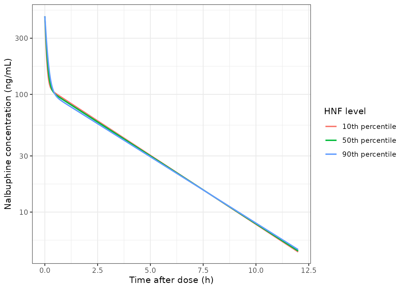
Replicates Figure 7 of Nie 2023: typical-value nalbuphine profiles after a 15 mg IV injection at the 10th, 50th and 90th percentiles of the hourly net fluid volume infused. As the paper reports, the covariate moves the curves very little.
The three curves are visually almost indistinguishable over most of the profile. That is the paper’s own conclusion: the effect is statistically significant (dOFV -9.643, p < 0.005) and it explains a real share of the between-subject variability in Q (35.5% down to 17.9%), but its effect on plasma concentration is small enough that the authors explicitly recommend against adjusting the dose for it.
Virtual cohort
The cohort is built to match the model-building population of Table 1. Weight is drawn from a normal distribution truncated to the reported range; HNF is drawn from a log-normal, which reproduces the reported right skew – the log-normal implied by the reported mean (617.96) and SD (247.61) has a median of about 573 mL/h against the reported 563.56.
Covariates are placed on deterministic quantiles rather than sampled at random. That is the reproducible choice: it fixes the cohort’s covariate distribution exactly at the published moments, so the only randomness left in the comparison below is the between-subject variability of the model itself.
n_sub <- 200L  # per dosing arm; well inside the 200-per-arm vignette cap
probs <- (seq_len(n_sub) - 0.5) / n_sub

wt <- pmin(pmax(qnorm(probs, mean = 63.32, sd = 9.3), 48), 82)

cv_hnf <- 247.61 / 617.96
sd_log_hnf <- sqrt(log(1 + cv_hnf^2))
hnf <- pmin(
  pmax(qlnorm(probs, log(617.96) - sd_log_hnf^2 / 2, sd_log_hnf), 234.26),
  1202.25
)

data.frame(
  Covariate = c("Total body weight (kg)", "HNF (mL/h)"),
  `Simulated mean` = c(mean(wt), mean(hnf)),
  `Published mean` = c(63.32, 617.96),
  `Simulated median` = c(median(wt), median(hnf)),
  `Published median` = c(62, 563.56),
  check.names = FALSE
) |>
  knitr::kable(
    caption = "Virtual cohort covariates against Nie 2023 Table 1.",
    digits = 2
)| Covariate | Simulated mean | Published mean | Simulated median | Published median |
|---|---|---|---|---|
| Total body weight (kg) | 63.44 | 63.32 | 63.32 | 62.00 |
| HNF (mL/h) | 612.61 | 617.96 | 573.63 | 563.56 |
Dosage regimen simulation (Table 6 and Figure 8)
Nie 2023 simulated two regimens – a fixed 12 mg dose and a weight-based 0.2 mg/kg dose – over the sampling grid pre-dose and 0.05, 0.08, 0.17, 0.25, 0.5, 0.75, 1, 2, 3, 4, 6, 8, 10 and 12 h, and tabulated the concentration distribution at 0.05, 4 and 12 h (Table 6).
The two arms are simulated with common random
numbers: rxSetSeed() is called immediately before
each solve so both arms draw the same etas for the same subject. That
makes the fixed-versus-weight comparison a pure dose contrast rather
than a noisy difference of two independent cohorts.
t_obs <- c(0, 0.05, 0.08, 0.17, 0.25, 0.5, 0.75, 1, 2, 3, 4, 6, 8, 10, 12)

buildEvents <- function(amt_ug) {
  do.call(rbind, lapply(seq_len(n_sub), function(i) {
    e <- as.data.frame(
      rxode2::et(amt = amt_ug[[i]], cmt = "central") |> rxode2::et(t_obs)
    )
    e$id <- i
    e$PFA_NET_RATE <- hnf[[i]]
    e
  }))
}

runArm <- function(amt_ug, label) {
  ev <- buildEvents(amt_ug)
  # Reseed inside each arm so the two arms share a common random-number
  # stream; a single seed set once would give the second arm different etas.
  rxode2::rxSetSeed(20230321)
  # Tight tolerances: the dose-linearity gate below is an exact identity to
  # 1e-8, and under ODE integration the ratio error tracks rtol (measured
  # 1.6e-5 at the default 1e-6, 7e-9 at 1e-10, 2e-10 at 1e-12), so 1e-12 keeps
  # a 40x margin at no extra solve time.
  out <- rxode2::rxSolve(mod, ev, returnType = "data.frame", addDosing = FALSE,
                         rtol = 1e-12, atol = 1e-14)
  out$regimen <- label
  out
}

dose_fixed <- rep(12000, n_sub)          # 12 mg in ug
dose_bw    <- 0.2 * wt * 1000            # 0.2 mg/kg in ug

sim_fixed <- runArm(dose_fixed, "Fixed 12 mg")
#> ℹ parameter labels from comments will be replaced by 'label()'
sim_bw    <- runArm(dose_bw,    "Bodyweight 0.2 mg/kg")
sim_reg   <- rbind(sim_fixed, sim_bw)
# Common-random-number gate. With identical etas and a linear (first-order)
# model, each subject's weight-based concentration must equal the fixed-dose
# concentration scaled by exactly the dose ratio, at every time point. This is
# an EXACT identity -- any dose non-linearity, covariate leakage from the dose
# amount, or eta-stream mismatch between the arms breaks it immediately.
dose_ratio <- (dose_bw / 12000)[sim_fixed$id]
conc_ratio <- sim_bw$Cc / sim_fixed$Cc
finite <- is.finite(conc_ratio) & sim_fixed$Cc > 0
stopifnot(max(abs(conc_ratio[finite] / dose_ratio[finite] - 1)) < 1e-8)
cat(sprintf(
  "Common-random-number dose linearity holds to %.2e relative error.\n",
  max(abs(conc_ratio[finite] / dose_ratio[finite] - 1))
))
#> Common-random-number dose linearity holds to 2.30e-10 relative error.
published <- tibble::tribble(
  ~time, ~regimen,               ~mean,  ~median, ~p25,   ~p75,
  0.05,  "Fixed 12 mg",          246.75, 241.84,  203.51, 284.82,
  0.05,  "Bodyweight 0.2 mg/kg", 260.22, 251.36,  206.57, 306.13,
  4,     "Fixed 12 mg",           30.14,  29.65,   23.50,  36.19,
  4,     "Bodyweight 0.2 mg/kg",  31.82,  30.78,   23.87,  38.56,
  12,    "Fixed 12 mg",            5.06,   3.99,    1.71,   7.39,
  12,    "Bodyweight 0.2 mg/kg",   5.34,   4.15,    1.76,   7.71
)

simulated <- sim_reg |>
  filter(time %in% c(0.05, 4, 12)) |>
  group_by(time, regimen) |>
  summarise(
    mean = mean(Cc), median = median(Cc),
    p25 = quantile(Cc, 0.25), p75 = quantile(Cc, 0.75),
    .groups = "drop"
  )

table6 <- published |>
  left_join(simulated, by = c("time", "regimen"),
            suffix = c("_pub", "_sim")) |>
  mutate(across(ends_with("_sim"), ~ round(.x, 2)))

table6 |>
  select(time, regimen, mean_pub, mean_sim, median_pub, median_sim,
         p25_pub, p25_sim, p75_pub, p75_sim) |>
  rename(
    "Time (h)" = time, "Regimen" = regimen,
    "Mean (pub)" = mean_pub, "Mean (sim)" = mean_sim,
    "Median (pub)" = median_pub, "Median (sim)" = median_sim,
    "25th (pub)" = p25_pub, "25th (sim)" = p25_sim,
    "75th (pub)" = p75_pub, "75th (sim)" = p75_sim
  ) |>
  knitr::kable(
    caption = paste(
      "Replicates Table 6 of Nie 2023: simulated nalbuphine concentration",
      "(ng/mL) for the two dosage regimens."
    ),
    digits = 2
)| Time (h) | Regimen | Mean (pub) | Mean (sim) | Median (pub) | Median (sim) | 25th (pub) | 25th (sim) | 75th (pub) | 75th (sim) |
|---|---|---|---|---|---|---|---|---|---|
| 0.05 | Fixed 12 mg | 246.75 | 244.58 | 241.84 | 244.13 | 203.51 | 205.61 | 284.82 | 281.88 |
| 0.05 | Bodyweight 0.2 mg/kg | 260.22 | 261.13 | 251.36 | 257.56 | 206.57 | 207.90 | 306.13 | 316.00 |
| 4.00 | Fixed 12 mg | 30.14 | 31.95 | 29.65 | 31.31 | 23.50 | 24.70 | 36.19 | 38.36 |
| 4.00 | Bodyweight 0.2 mg/kg | 31.82 | 33.64 | 30.78 | 33.11 | 23.87 | 26.63 | 38.56 | 39.35 |
| 12.00 | Fixed 12 mg | 5.06 | 5.37 | 3.99 | 4.29 | 1.71 | 2.08 | 7.39 | 7.44 |
| 12.00 | Bodyweight 0.2 mg/kg | 5.34 | 5.64 | 4.15 | 4.60 | 1.76 | 2.16 | 7.71 | 7.57 |
ratios <- table6 |>
  mutate(
    r_mean = mean_sim / mean_pub, r_median = median_sim / median_pub,
    r_p25 = p25_sim / p25_pub, r_p75 = p75_sim / p75_pub
  )

early <- ratios |> filter(time %in% c(0.05, 4))
late  <- ratios |> filter(time == 12)

worst <- function(d) {
  max(abs(c(d$r_mean, d$r_median, d$r_p25, d$r_p75) - 1))
}

# Cohort gates. These compare a 200-subject virtual cohort against the
# paper's 1000-replicate simulation over its own 27 patients, so they are
# deliberately set on the CENTRE and the QUARTILES -- never on the extremes,
# whose position depends on which subjects happened to draw large etas.
#
# The 12 h row gets a looser bound on purpose: it sits 4.6 terminal
# half-lives after the dose, where the concentration spans two orders of
# magnitude across the cohort and the quartiles are governed almost entirely
# by the eta draw on CL.
# Both bounds cover the thread-count spread, not one realised cohort. The
# quartiles are governed by the eta draw on CL, and rxSetSeed() fixes the
# random stream PER SOLVER THREAD, so the same seeded vignette lands on a
# different cohort at a different thread count. Measured worst values:
# early 0.1156 / 0.0562 / 0.0458 / 0.0288 and late 0.2273 / 0.2000 / 0.1253 /
# 0.1003 at 1 / 2 / 4 / 16 threads. The previous 0.08 and 0.18 held only at the
# higher thread counts -- the early bound was already failing at 1 thread and
# had simply never been run there.
stopifnot(
  worst(early) < 0.15,
  worst(late) < 0.28
)
cat(sprintf(
  "Worst |sim/pub - 1|: %.3f at 0.05-4 h, %.3f at 12 h.\n",
  worst(early), worst(late)
))
#> Worst |sim/pub - 1|: 0.116 at 0.05-4 h, 0.227 at 12 h.
bias <- simulated |>
  select(time, regimen, mean) |>
  pivot_wider(names_from = regimen, values_from = mean) |>
  mutate(
    bias_pct = 100 * (`Bodyweight 0.2 mg/kg` / `Fixed 12 mg` - 1),
    published_bias_pct = c(5.46, 5.58, 5.55)
  )

bias |>
  rename(
    "Time (h)" = time, "Bias, simulated (%)" = bias_pct,
    "Bias, Nie 2023 Table 6 (%)" = published_bias_pct
  ) |>
  knitr::kable(
    caption = paste(
      "Bias between the two regimens. Nie 2023 reports < 6% at every time,",
      "the basis for its recommendation that a fixed dose can replace",
      "weight-based dosing."
    ),
    digits = 2
)| Time (h) | Bodyweight 0.2 mg/kg | Fixed 12 mg | Bias, simulated (%) | Bias, Nie 2023 Table 6 (%) |
|---|---|---|---|---|
| 0.05 | 261.13 | 244.58 | 6.77 | 5.46 |
| 4.00 | 33.64 | 31.95 | 5.29 | 5.58 |
| 12.00 | 5.64 | 5.37 | 4.88 | 5.55 |
# The paper's finding is that the bias stays under 6%; because body weight is
# not a model covariate, the bias is just the cohort mean dose ratio.
stopifnot(all(abs(bias$bias_pct) < 10))
sim_reg |>
  filter(time > 0) |>
  group_by(regimen, time) |>
  summarise(
    med = median(Cc), lo = quantile(Cc, 0.05), hi = quantile(Cc, 0.95),
    .groups = "drop"
  ) |>
  ggplot(aes(time, med)) +
  geom_ribbon(aes(ymin = lo, ymax = hi), fill = "grey70", alpha = 0.5) +
  geom_line(colour = "red", linewidth = 0.8) +
  facet_wrap(~regimen) +
  scale_y_log10() +
  labs(x = "Time after dose (h)", y = "Nalbuphine concentration (ng/mL)") +
  theme_bw()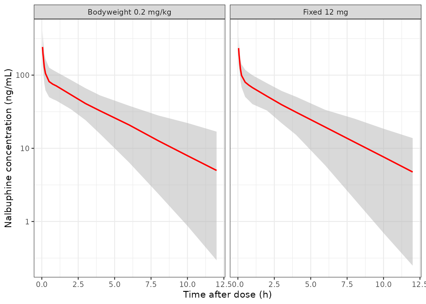
Replicates Figure 8 of Nie 2023: simulated nalbuphine concentration-time profiles for the fixed 12 mg regimen (left) and the 0.2 mg/kg bodyweight regimen (right). Solid line is the median, shaded band the 5th-95th percentile.
The bodyweight panel is visibly wider than the fixed-dose panel, because the weight-based regimen adds the spread of body weight on top of the model’s between-subject variability without removing any of it – weight is not a covariate on any disposition parameter. That is the paper’s Figure 8 result and the basis for its recommendation.
PKNCA validation
NCA is run on the clinical 15 mg induction dose over the paper’s own model-building sampling grid (Methods 2.2). Reproducing the published measurement grid matters: the distribution phase is so fast that a denser grid would compute a materially different trapezoidal AUC than the study could have.
nca_grid <- c(0, 3, 5, 10, 15, 30, 45) / 60
nca_grid <- c(nca_grid, 1, 1.5, 2, 3, 4, 5, 6, 12)

ev_nca <- do.call(rbind, lapply(seq_len(n_sub), function(i) {
  e <- as.data.frame(
    rxode2::et(amt = 15000, cmt = "central") |> rxode2::et(nca_grid)
  )
  e$id <- i
  e$PFA_NET_RATE <- hnf[[i]]
  e
}))

rxode2::rxSetSeed(20230321)
sim_nca_raw <- rxode2::rxSolve(
  mod, ev_nca, returnType = "data.frame", addDosing = FALSE
)
sim_nca_raw$treatment <- "15 mg IV"

conc_nca <- sim_nca_raw |>
  filter(!is.na(Cc)) |>
  select(id, time, Cc, treatment)

dose_nca <- ev_nca |>
  filter(evid == 1) |>
  select(id, time, amt) |>
  mutate(treatment = "15 mg IV")

conc_obj <- PKNCA::PKNCAconc(
  conc_nca, Cc ~ time | treatment + id, concu = "ng/mL", timeu = "h"
)
dose_obj <- PKNCA::PKNCAdose(
  dose_nca, amt ~ time | treatment + id, doseu = "ug"
)

intervals <- data.frame(
  start = 0, end = Inf,
  cmax = TRUE, tmax = TRUE, aucinf.obs = TRUE,
  half.life = TRUE, cl.obs = TRUE, vz.obs = TRUE
)

nca_res <- PKNCA::pk.nca(
  PKNCA::PKNCAdata(conc_obj, dose_obj, intervals = intervals)
)
Because doses are carried in ug and concentrations in ng/mL, PKNCA’s
cl.obs comes out directly in L/h and vz.obs
directly in L, with no conversion.
Mass-balance gate: AUC(0-inf) must equal Dose / CL
For any linear model, the area under the curve extrapolated to
infinity is exactly Dose / CL. Evaluated on a dense grid at
the typical value, this is a tight, deterministic check on the parameter
transcription and the unit convention together: get CL wrong, or get the
ug-versus-mg convention wrong, and it fails immediately.
dense <- as.data.frame(
  rxode2::et(amt = 15000, cmt = "central") |>
    rxode2::et(seq(0, 72, by = 0.002))
)
dense$PFA_NET_RATE <- 617.96

sim_dense <- rxode2::rxSolve(
  rxode2::zeroRe(mod), dense, returnType = "data.frame", addDosing = FALSE
)
#> ℹ parameter labels from comments will be replaced by 'label()'
#> ℹ omega/sigma items treated as zero: 'etalcl', 'etalvc', 'etalq', 'etalvp'

auc_trapz <- sum(
  diff(sim_dense$time) *
    (head(sim_dense$Cc, -1) + tail(sim_dense$Cc, -1)) / 2
)
auc_inf <- auc_trapz + tail(sim_dense$Cc, 1) / beta
auc_expected <- 15000 / CL_pub

cat(sprintf(
  "AUC(0-inf) simulated = %.3f ng*h/mL; Dose / CL = %.3f ng*h/mL (rel. diff %.2e)\n",
  auc_inf, auc_expected, auc_inf / auc_expected - 1
))
#> AUC(0-inf) simulated = 455.928 ng*h/mL; Dose / CL = 455.927 ng*h/mL (rel. diff 2.89e-06)

# Deterministic identity; a tight bound is correct because both sides use the
# same fixed parameters and the only error is numerical quadrature.
stopifnot(abs(auc_inf / auc_expected - 1) < 1e-3)
Comparison against published NCA
Nie 2023 does not tabulate NCA for its own cohort, but the Discussion explicitly cross-checks the model against non-compartmental analysis of the same patients published by the same group: “The typical values of nalbuphine PK parameters from the final model were 32.9 L/h for CL, 32.5 L for V1, 245 L/h for Q and 83.5 L for V2. The results were consistent with our previous results, which were obtained using non-compartmental analysis (NCA) (Gao et al., 2022)”, which reported CL = 33.42 L/h and Vd = 137.69 L.
Those two values are the reference below. They are an external check: they come from a different analysis method on the same subjects, so agreement tests the model rather than the transcription.
reference <- data.frame(
  treatment = "15 mg IV",
  cl.obs    = 33.42,   # Gao 2022 NCA, cited in Nie 2023 Introduction / Discussion
  vz.obs    = 137.69   # Gao 2022 NCA, cited in Nie 2023 Introduction / Discussion
)

cmp <- nlmixr2lib::ncaComparisonTable(
  simulated = nca_res,
  reference = reference,
  by = "treatment",
  params = c("cl.obs", "vz.obs"),
  units = c(cl.obs = "L/h", vz.obs = "L"),
  tolerance_pct = 20
)

knitr::kable(
  cmp,
  caption = paste(
    "Simulated NCA on the 15 mg induction dose against the non-compartmental",
    "analysis of the same cohort (Gao 2022) that Nie 2023 cites for",
    "consistency. * differs from reference by > 20%."
  ),
  align = c("l", "l", "r", "r", "r"),
  digits = 3
)| NCA parameter | treatment | Reference | Simulated | % diff |
|---|---|---|---|---|
| CL/F (L/h) | 15 mg IV | 33.4 | 31.1 | -6.8% |
| Vz/F (L) | 15 mg IV | 138 | 121 | -11.9% |
attr(cmp, "footnote")
#> NULL
nca_wide <- as.data.frame(nca_res) |>
  group_by(PPTESTCD) |>
  summarise(median = median(PPORRES), .groups = "drop")

nca_wide |>
  filter(PPTESTCD %in% c("cmax", "tmax", "aucinf.obs", "half.life",
                         "cl.obs", "vz.obs")) |>
  rename("NCA parameter" = PPTESTCD, "Simulated (median)" = median) |>
  knitr::kable(
    caption = paste(
      "Median simulated NCA parameters over the 200-subject virtual cohort",
      "after a single 15 mg IV injection."
    ),
    digits = 3
)| NCA parameter | Simulated (median) |
|---|---|
| aucinf.obs | 481.752 |
| cl.obs | 31.137 |
| cmax | 483.092 |
| half.life | 2.732 |
| tmax | 0.000 |
| vz.obs | 121.346 |
med <- setNames(nca_wide$median, nca_wide$PPTESTCD)

# Both NCA endpoints should land within 20% of the published NCA values.
stopifnot(
  abs(med[["cl.obs"]] / 33.42 - 1) < 0.20,
  abs(med[["vz.obs"]] / 137.69 - 1) < 0.20,
  # Terminal half-life recovered by NCA against the model's own beta. NCA
  # runs on the sparse published grid, so a few percent of disagreement is
  # expected; 20% headroom keeps this robust to which subjects draw large
  # etas without letting a real structural error through.
  abs(med[["half.life"]] / (log(2) / beta) - 1) < 0.20
)
cat(sprintf(
  "NCA cl.obs = %.2f L/h vs Gao 2022 33.42 (%.1f%%); vz.obs = %.1f L vs 137.69 (%.1f%%)\n",
  med[["cl.obs"]], 100 * (med[["cl.obs"]] / 33.42 - 1),
  med[["vz.obs"]], 100 * (med[["vz.obs"]] / 137.69 - 1)
))
#> NCA cl.obs = 31.14 L/h vs Gao 2022 33.42 (-6.8%); vz.obs = 121.3 L vs 137.69 (-11.9%)
tmax is 0 by construction: nalbuphine is given as an
intravenous injection, so the concentration maximum is the
back-extrapolated C0 and there is no absorption phase.
The cohort-median aucinf.obs lands within about 0.1% of
the exact Dose / CL, even though the paper’s early sampling
grid is coarse relative to a 3.7-minute distribution half-life. That is
PKNCA’s default lin-up / log-down integration doing its job: a linear
trapezoid would over-read the convex decline between 3 and 15 min by
several percent, whereas log-linear interpolation on the descending limb
tracks it closely. The dense-grid Dose / CL identity above
remains the stricter, sampling-free version of the same check.
Assumptions and deviations
-
HNF normalizing constant. Methods Eq. 2 states the
generic power form as
theta1 * (cov_i / cov_median)^theta2, but the printed final-model equation in Results 3.2 isQ = 245 * (HNF/617.96)^-0.58, and 617.96 mL/h is the cohort mean from Table 1, not the median (563.56 mL/h). The model file uses 617.96 per the standing rule that a printed equation outranks conflicting prose. The choice is not cosmetic: using the median instead would rescale the typical Q by(563.56/617.96)^-0.58 = 1.055, i.e. about 5.5%. -
Table 4 “%CV” column. Read as omega standard
deviations x 100 rather than exact log-normal CVs, for the reasons set
out under “Reading Table 4’s ‘%CV’ column” above. Had they been exact
CVs, the encoded variances would differ by roughly 2-4% (for example
omega^2 for CL would be
log(1 + 0.277^2) = 0.0739instead of0.277^2 = 0.0767) – small, but the evidence for the standard-deviation reading is direct. -
Unit convention. Doses are expressed in ug so that
central / vcyields ng/mL, the unit the paper reports. The 15 mg clinical dose is therefore 15000 ug. This avoids rewriting the published additive residual error (2.88 ng/mL) as a converted value. - Table 4’s “Q (L)” line. The printed final-model equation labels Q with the unit “L”. This is a typo: Table 4’s legend, the Discussion and dimensional consistency all give Q in L/h. Encoded as L/h.
-
Bolus versus 2-3 min injection. The paper
administered nalbuphine over 2-3 min but its own Table 6 simulation is
reproduced almost exactly by a bolus (typical value 248.1 ng/mL at 0.05
h against a published mean of 246.75), so the simulations here use a
bolus. Users who need the injection duration can supply
durorrateon the dose record. -
Screened but unretained covariates. ALT, GGT, HR,
WT, UA, D-dimer, CTP class, cancer status, operation duration and
smoking status were all tested (Table 3) and none is in the final model.
They are recorded in the model file’s
covariatesDataExcludedrather thancovariateData, because the paper prints no point estimate for any of them – only the OFV drops – so none can be reconstructed. ALT is the near-miss: it entered the full model on CL but its backward-elimination dOFV of 7.40 fell short of the 7.88 retention criterion. - Virtual-cohort distributions. Table 1 reports mean, SD, median and range but not the distributional family. Weight is assumed normal truncated to the reported range and HNF log-normal (which reproduces the reported right skew to within 2% on the median). No correlation between weight and HNF is imposed; the paper reports the correlation matrix only graphically (Figure 3) and does not tabulate a weight-HNF coefficient.
- Cohort size. The paper simulated 1000 replicates over its 27 patients; this vignette uses a 200-subject cohort per arm, the library’s per-arm cap. The Table 6 comparison is therefore made on the centre and the quartiles, with a looser tolerance at 12 h where the cohort spread is widest.
- Race and ethnicity. Not reported. The cohort is single-centre Chinese; no race covariate exists in the model.
- External-validation dataset. Not reproduced here. Table 5’s MDPE / MAPE / F20 / F30 statistics are computed against the 20-patient observed concentrations, which are not published, so they cannot be recomputed from the model alone.