Palbociclib PK and neutropenia (Courlet 2022)
Source:vignettes/articles/Courlet_2022_palbociclib.Rmd
Courlet_2022_palbociclib.RmdModel and source
Courlet et al. (2022) modelled oral palbociclib pharmacokinetics and the time course of absolute neutrophil counts (ANC) in 44 women treated for advanced breast cancer in routine care at Lausanne University Hospital (OpTAT study). Concentrations came from routine visits plus rich sampling over a dosing interval, including samples taken during the OFF-treatment week.
The paper reports two final models, and both are packaged:
-
Courlet_2022_palbociclib– the final PK-only model (Supplementary Table S1). It is the model the paper uses for its proton-pump-inhibitor (PPI) simulation (Figure 3). -
Courlet_2022_palbociclib_anc– the final PK/PD model (Table 2), in which the PK parameters were re-estimated together with the PD parameters. It is the model behind every neutropenia simulation (Figures 4 and 5).
The PK model is two-compartment with first-order absorption, an absorption lag time and first-order elimination. Apparent clearance takes a separately estimated value when palbociclib is taken under fasting conditions (or with a light meal) together with a PPI. PPI use with a meal has no effect. The PD model is Friberg’s semi-mechanistic myelosuppression model with an Emax drug effect on proliferation. EC50 was fixed to the literature value because it could not be estimated from the narrow dose range.
- Citation: Courlet P, Cardoso E, Bandiera C, Stravodimou A, Zurcher JP, Chtioui H, Locatelli I, Decosterd LA, Darnaud L, Blanchet B, Alexandre J, Wagner AD, Zaman K, Schneider MP, Guidi M, Csajka C. (2022). Population Pharmacokinetics of Palbociclib and Its Correlation with Clinical Efficacy and Safety in Patients with Advanced Breast Cancer. Pharmaceutics 14(7):1317. doi:10.3390/pharmaceutics14071317.
- Article: https://doi.org/10.3390/pharmaceutics14071317 (open access)
- Supplement: https://www.mdpi.com/article/10.3390/pharmaceutics14071317/s1 (Table S1, the final PK-only model; Table S2, the Cox analysis)
Population
The analysis used 255 palbociclib concentrations (2.0-159.0 ng/mL, median 5 per patient) and 1174 ANC values (40 before palbociclib started) from 44 women. The median daily dose was 100 mg (range 75-125 mg), given 21 days on and 7 days off. Table 1 of the paper, median [IQR] or n (%):
| Characteristic | Value |
|---|---|
| Age (years) | 65 [55-75] |
| Body weight (kg) | 67 [61-80] |
| AST / ALT (U/L) | 23 [19-28] / 20 [15-27] |
| Total bilirubin (umol/L) | 5 [4-7] |
| Albumin (g/L) | 43 [41-45] |
| Alkaline phosphatase (U/L) | 61 [49-81] |
| GGT (U/L) | 29 [18-51] |
| Creatinine (umol/L) | 71 [63-85] |
| eGFR, Cockcroft-Gault (mL/min/1.73 m^2) | 71 [54-98] |
| Fasting administration (per concentration) | 54 (21%) |
| PPI co-administration (per concentration) | 78 (31%) |
| Fulvestrant co-administration (per ANC) | 822 (70%) |
The same information is available programmatically via
readModelDb("Courlet_2022_palbociclib_anc")()$population.
Source trace
| Model element | PK-only model | PK/PD model | Source |
|---|---|---|---|
| Two-compartment PK, first-order absorption with lag | – | – | Section 3.2.1 |
lka |
0.73 /h | 0.8 /h | Table S1 / Table 2 |
ltlag |
1.9 h | 2.0 h | Table S1 / Table 2 |
lcl (fed, or no PPI) |
68 L/h | 67 L/h | Table S1 / Table 2 |
lcl_ppifasted (fasting + PPI) |
106 L/h | 131 L/h | Table S1 / Table 2; Section 3.2.1 |
lvc |
2730 L | 2800 L | Table S1 / Table 2 |
lq |
5.1 L/h | 7 L/h | Table S1 / Table 2 |
lvp |
717 L | 704 L | Table S1 / Table 2 |
etalka, etalcl, etalvc
|
126%, 30%, 36% CV | 125%, 29%, 32% CV | Table S1 / Table 2 |
propSd |
18% | 18% | Table S1 / Table 2 |
Friberg chain, ktr = (n + 1) / MTT,
kprol = ktr = kcirc
|
– | – | Section 2.3.2; Figure 1 |
E = Emax * C / (EC50 + C) on proliferation |
– | – | Equation 2; Figure 1 |
Feedback (Base / Circ)^gamma
|
– | – | Section 2.3.2; Figure 1 |
lcirc0 |
– | 4.1 G/L | Table 2 |
lmtt |
– | 122 h | Table 2 |
lemax |
– | 0.22 | Table 2 |
lec50 (fixed) |
– | 40.1 ng/mL | Table 2; Section 3.2.2 |
lgamma |
– | 0.13 | Table 2 |
etalcirc0, etalmtt, etalemax,
etalec50
|
– | 35%, 12%, 15%, 93% CV | Table 2 |
expSd_ANC (additive on log ANC) |
– | 0.31 | Table 2; Section 2.3.2 |
Event tables
The label regimen is 125 mg once daily for 21 days of each 28-day
cycle. The PK/PD model has two endpoints (Cc and
ANC), so its observation rows carry dvid = 1;
both outputs come back as columns. The neutropenia measures below use
the circulating-neutrophil state circ (equal to
ANC without residual error).
dose_times <- function(n_cycles = 3, off = 7) {
  unlist(lapply(seq_len(n_cycles) - 1, function(cyc) cyc * (21 + off) * 24 + (0:20) * 24))
}
make_events <- function(ids, dose_mg = 125, off = 7, n_cycles = 3,
                        obs_times = seq(0, 84 * 24, by = 12)) {
  do.call(rbind, lapply(ids, function(i) {
    rbind(
      data.frame(id = i, time = dose_times(n_cycles, off), amt = dose_mg, evid = 1L, cmt = "depot", dvid = NA_integer_),
      data.frame(id = i, time = obs_times, amt = 0, evid = 0L, cmt = "central", dvid = 1L)
    )
  })) |>
    dplyr::arrange(id, time, dplyr::desc(evid))
}
mod_pk <- readModelDb("Courlet_2022_palbociclib")
mod_pd <- readModelDb("Courlet_2022_palbociclib_anc")
Pharmacokinetics
Typical steady state and PKNCA
Day 21 of the first cycle is used as steady state. Both models are solved at their typical values for a patient taking 125 mg with a meal and for one taking it fasting with a PPI.
scen <- data.frame(
  id = 1:4,
  model = c("PK-only", "PK-only", "PK/PD", "PK/PD"),
  condition = rep(c("Meal, no PPI", "Fasting + PPI"), 2),
  CONMED_PPI = c(0, 1, 0, 1),
  FED = c(1, 0, 1, 0),
  cl = c(68, 106, 67, 131)
)
obs_ss <- sort(unique(c(seq(0, 504, by = 0.25))))
solve_typ <- function(mod, rows, keep_dvid) {
  ev <- make_events(rows$id, n_cycles = 1, obs_times = obs_ss) |>
    dplyr::left_join(rows[, c("id", "CONMED_PPI", "FED")], by = "id")
  # The PK-only model has a single endpoint and no dvid.
  if (!keep_dvid) ev$dvid <- NULL
  rxode2::rxSolve(rxode2::zeroRe(mod), ev, returnType = "data.frame",
                  atol = 1e-10, rtol = 1e-10, useLinCmt = FALSE) |>
    as.data.frame()
}
sim_ss <- dplyr::bind_rows(
  solve_typ(mod_pk, scen[scen$model == "PK-only", ], keep_dvid = FALSE),
  solve_typ(mod_pd, scen[scen$model == "PK/PD", ], keep_dvid = TRUE)
) |>
  dplyr::left_join(scen[, c("id", "model", "condition")], by = "id") |>
  dplyr::mutate(treatment = paste(model, condition, sep = ": "))
#> ℹ parameter labels from comments will be replaced by 'label()'
#> ℹ omega/sigma items treated as zero: 'etalka', 'etalcl', 'etalvc'
#> Warning: multi-subject simulation without without 'omega'
#> ℹ parameter labels from comments will be replaced by 'label()'
#> ℹ omega/sigma items treated as zero: 'etalka', 'etalcl', 'etalvc', 'etalcirc0', 'etalmtt', 'etalemax', 'etalec50'
#> Warning: multi-subject simulation without without 'omega'
conc_ss <- sim_ss |>
  dplyr::filter(!is.na(Cc), time >= 480, time <= 504) |>
  dplyr::mutate(time = time - 480) |>
  dplyr::select(id, treatment, time, Cc)
dose_ss <- scen |>
  dplyr::mutate(treatment = paste(model, condition, sep = ": "), time = 0, amt = 125) |>
  dplyr::select(id, treatment, time, amt)
conc_obj <- PKNCA::PKNCAconc(conc_ss, Cc ~ time | treatment + id, concu = "ng/mL", timeu = "h")
dose_obj <- PKNCA::PKNCAdose(dose_ss, amt ~ time | treatment + id, doseu = "mg")
intervals <- data.frame(start = 0, end = 24, cmax = TRUE, tmax = TRUE, cmin = TRUE, auclast = TRUE)
nca_res <- PKNCA::pk.nca(PKNCA::PKNCAdata(conc_obj, dose_obj, intervals = intervals))
nca_wide <- as.data.frame(nca_res$result) |>
  dplyr::select(treatment, PPTESTCD, PPORRES) |>
  tidyr::pivot_wider(names_from = PPTESTCD, values_from = PPORRES) |>
  dplyr::left_join(
    scen |> dplyr::transmute(treatment = paste(model, condition, sep = ": "), auc_closed = 125000 / cl),
    by = "treatment"
  )
nca_wide |>
  dplyr::select(treatment, cmax, tmax, cmin, auclast, auc_closed) |>
  dplyr::rename(
    "Model: condition" = treatment,
    "Cmax,ss (ng/mL)" = cmax,
    "Tmax (h)" = tmax,
    "Cmin,ss (ng/mL)" = cmin,
    "AUC0-24,ss (ng*h/mL)" = auclast,
    "Dose/CL (ng*h/mL)" = auc_closed
  ) |>
knitr::kable(digits = 1, caption = "Typical-value steady-state NCA on day 21 of the first cycle, 125 mg once daily.")| Model: condition | Cmax,ss (ng/mL) | Tmax (h) | Cmin,ss (ng/mL) | AUC0-24,ss (ng*h/mL) | Dose/CL (ng*h/mL) |
|---|---|---|---|---|---|
| PK-only: Fasting + PPI | 65.8 | 5.5 | 31.6 | 1176.6 | 1179.2 |
| PK-only: Meal, no PPI | 92.6 | 5.5 | 57.9 | 1829.6 | 1838.2 |
| PK/PD: Fasting + PPI | 56.9 | 5.2 | 23.0 | 953.3 | 954.2 |
| PK/PD: Meal, no PPI | 93.9 | 5.5 | 59.2 | 1860.3 | 1865.7 |
Figure 3: fasting with a PPI
Section 3.2.3 reports a 35% lower median exposure when palbociclib is taken fasting with a PPI than with a meal and no PPI (PK-only model). The exposure ratio of the two typical patients is the clearance ratio:
auc_pk <- setNames(nca_wide$auclast, nca_wide$treatment)
pct_lower <- 100 * (1 - auc_pk[["PK-only: Fasting + PPI"]] / auc_pk[["PK-only: Meal, no PPI"]])
pct_lower
#> [1] 35.68865
# Paper: 35% (1 - 68/106 = 35.8%). A PPI effect on the wrong arm, or the PK/PD
# clearances (1 - 67/131 = 49%), fails this.
stopifnot(abs(pct_lower - 35) < 2)
The paper simulated 1000 patients per condition. The figure below uses 200 per condition at steady state with all PK random effects.
rxode2::rxSetSeed(2022)
ev_fig3 <- dplyr::bind_rows(
  make_events(1:200, n_cycles = 1, obs_times = seq(480, 504, by = 0.5)) |>
    dplyr::mutate(CONMED_PPI = 0, FED = 1, condition = "Meal, no PPI"),
  make_events(201:400, n_cycles = 1, obs_times = seq(480, 504, by = 0.5)) |>
    dplyr::mutate(CONMED_PPI = 1, FED = 0, condition = "Fasting + PPI")
) |>
  dplyr::select(-dvid)
stopifnot(!anyDuplicated(unique(ev_fig3[, c("id", "time", "evid")])))
sim_fig3 <- rxode2::rxSolve(mod_pk, ev_fig3, keep = "condition", returnType = "data.frame") |>
  as.data.frame()
#> ℹ parameter labels from comments will be replaced by 'label()'
fig3_sum <- sim_fig3 |>
  dplyr::group_by(condition, time) |>
  dplyr::summarise(
    p025 = quantile(Cc, 0.025), p50 = median(Cc), p975 = quantile(Cc, 0.975),
    .groups = "drop"
  )
ggplot(fig3_sum, aes(time - 480, p50, colour = condition, fill = condition)) +
  geom_ribbon(aes(ymin = p025, ymax = p975), alpha = 0.2, colour = NA) +
  geom_line() +
  labs(x = "Time after dose (h)", y = "Palbociclib (ng/mL)", colour = NULL, fill = NULL) +
  theme_bw()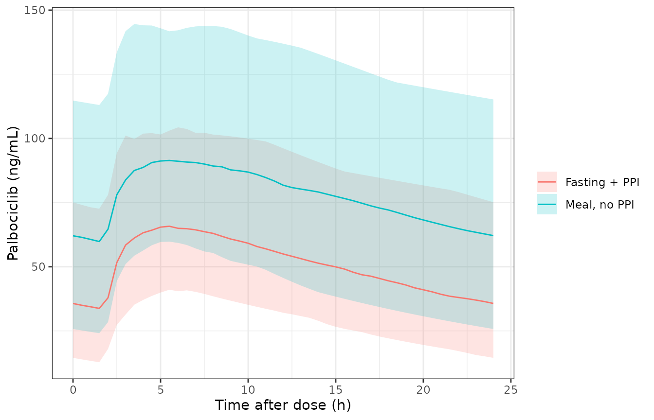
Replicates Figure 3 of Courlet 2022: steady-state palbociclib concentrations after 125 mg once daily (median and 95% prediction interval, 200 simulated patients per condition, PK-only model).
Pharmacodynamics
Figure 4: ANC over three cycles at 125, 100 and 75 mg
Section 3.2.3 reports, for 1000 simulated patients taking palbociclib with a meal, a grade 3 neutropenia incidence (at least one ANC below 1 G/L) of 36%, 29% and 21% at 125, 100 and 75 mg, and a grade 4 incidence (ANC below 0.5 G/L) of 5%, 3% and 2%, over three cycles. The nadir occurs about day 24 of the cycle (IQR 24-25) whatever the dose, and the median nadir is about 0.8 G/L in patients with grade 3 and 0.4 G/L in patients with grade 4 neutropenia. The cohorts below are 200 patients per dose, with all PK and PD random effects; incidence is computed on the individual ANC without residual error.
rxode2::rxSetSeed(1317)
regimens <- data.frame(
  regimen = c("125 mg 21/7", "100 mg 21/7", "75 mg 21/7", "125 mg 21/14"),
  dose = c(125, 100, 75, 125),
  off = c(7, 7, 7, 14)
)
n_arm <- 200
ev_fig4 <- dplyr::bind_rows(lapply(seq_len(nrow(regimens)), function(k) {
  make_events((k - 1) * n_arm + seq_len(n_arm),
    dose_mg = regimens$dose[k], off = regimens$off[k],
    obs_times = seq(0, 120 * 24, by = 12)
  ) |>
    dplyr::mutate(regimen = regimens$regimen[k])
})) |>
  dplyr::mutate(CONMED_PPI = 0, FED = 1)
stopifnot(!anyDuplicated(unique(ev_fig4[, c("id", "time", "evid")])))
sim_fig4 <- rxode2::rxSolve(mod_pd, ev_fig4, keep = "regimen", returnType = "data.frame", useLinCmt = FALSE) |>
  as.data.frame()
#> ℹ parameter labels from comments will be replaced by 'label()'
fig4_sum <- sim_fig4 |>
  dplyr::group_by(regimen, time) |>
  dplyr::summarise(
    p025 = quantile(ANC, 0.025), p50 = median(ANC), p975 = quantile(ANC, 0.975),
    .groups = "drop"
  ) |>
  dplyr::mutate(regimen = factor(regimen, levels = regimens$regimen))
ggplot(fig4_sum, aes(time / 24, p50)) +
  geom_ribbon(aes(ymin = p025, ymax = p975), alpha = 0.25) +
  geom_line() +
  geom_hline(yintercept = 1, linetype = "dotted", colour = "orange") +
  geom_hline(yintercept = 0.5, linetype = "dotted", colour = "red") +
  facet_wrap(~regimen) +
  labs(x = "Time (days)", y = "ANC (G/L)") +
  theme_bw()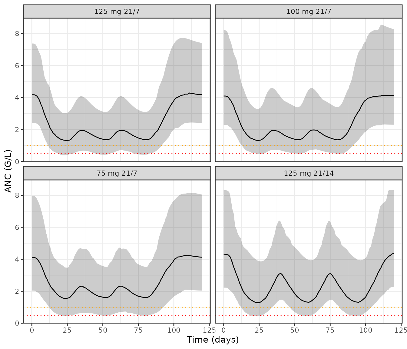
Replicates Figure 4 of Courlet 2022: ANC over three cycles (median and 95% prediction interval of the individual ANC without residual error, 200 patients per regimen). Dotted lines: grade 3 (1 G/L) and grade 4 (0.5 G/L) thresholds.
per_pat <- sim_fig4 |>
  dplyr::filter(regimen != "125 mg 21/14", time <= 84 * 24) |>
  dplyr::group_by(regimen, id) |>
  dplyr::summarise(
    nadir = min(circ),
    day_nadir = (time[which.min(circ)] %% (28 * 24)) / 24,
    .groups = "drop"
  )
incid <- per_pat |>
  dplyr::group_by(regimen) |>
  dplyr::summarise(
    g3_model = 100 * mean(nadir < 1),
    g4_model = 100 * mean(nadir < 0.5),
    day_nadir_model = median(day_nadir),
    .groups = "drop"
  ) |>
  dplyr::inner_join(
    data.frame(regimen = regimens$regimen[1:3], g3_paper = c(36, 29, 21), g4_paper = c(5, 3, 2)),
    by = "regimen"
  ) |>
  dplyr::arrange(match(regimen, regimens$regimen))
incid |>
  dplyr::select(regimen, g3_model, g3_paper, g4_model, g4_paper, day_nadir_model) |>
  dplyr::rename(
    "Regimen" = regimen,
    "Grade 3 incidence, model (%)" = g3_model,
    "Grade 3 incidence, paper (%)" = g3_paper,
    "Grade 4 incidence, model (%)" = g4_model,
    "Grade 4 incidence, paper (%)" = g4_paper,
    "Median nadir day of cycle, model" = day_nadir_model
  ) |>
knitr::kable(digits = 1, caption = "Neutropenia over three cycles: packaged model (200 patients per dose) versus Section 3.2.3 (1000 patients per dose).")| Regimen | Grade 3 incidence, model (%) | Grade 3 incidence, paper (%) | Grade 4 incidence, model (%) | Grade 4 incidence, paper (%) | Median nadir day of cycle, model |
|---|---|---|---|---|---|
| 125 mg 21/7 | 30.5 | 36 | 5.5 | 5 | 24.5 |
| 100 mg 21/7 | 28.0 | 29 | 3.5 | 3 | 24.5 |
| 75 mg 21/7 | 21.0 | 21 | 4.5 | 2 | 24.5 |
nadir_by_grade <- c(
  grade3 = median(per_pat$nadir[per_pat$nadir < 1 & per_pat$nadir >= 0.5]),
  grade4 = median(per_pat$nadir[per_pat$nadir < 0.5])
)
nadir_by_grade
#>    grade3    grade4
#> 0.7786639 0.4313569

stopifnot(
  # Binomial SD at n = 200 is about 3.4 points at 36% and 1.5 points at 5%; a
  # wrong Emax, EC50 or MTT unit moves these by tens of points.
  all(abs(incid$g3_model - incid$g3_paper) < 10),
  all(abs(incid$g4_model - incid$g4_paper) < 5),
  # Nadir about day 24 of each cycle (IQR 24-25).
  all(abs(incid$day_nadir_model - 24) <= 2),
  # Median nadir 0.8 G/L (grade 3) and 0.4 G/L (grade 4).
  abs(nadir_by_grade[["grade3"]] - 0.8) < 0.1
)
The grade 4 median nadir is computed from only a few percent of 200 patients per dose, so it is reported but not asserted.
Recovery after three cycles and the 21/14 schedule
Section 3.2.3 reports that after three standard cycles a median of 25 days (IQR 22-28) after the last dose was needed for ANC to return to its baseline. With a 14-day OFF period the ANC recovers better but has not yet reached baseline 14 days after the last dose.
last_dose <- (2 * 28 + 20) * 24
recov <- sim_fig4 |>
  dplyr::filter(regimen == "125 mg 21/7") |>
  dplyr::group_by(id) |>
  dplyr::summarise(
    base = circ[time == 0],
    t_rec = {
      tt <- time[time > last_dose & circ >= base]
      if (length(tt) == 0) Inf else (min(tt) - last_dose) / 24
    },
    .groups = "drop"
  )
# Patients still below baseline at the end of the 44-day follow-up count as
# Inf, so they sit in the upper tail rather than being dropped.
pct_not_recovered <- 100 * mean(is.infinite(recov$t_rec))
pct_not_recovered
#> [1] 2.5
recov_q <- quantile(recov$t_rec, c(0.25, 0.5, 0.75))
recov_q
#> 25% 50% 75%
#>  25  27  30
stopifnot(
  # Paper median 25 days; the model gives about 27. A unit slip on MTT
  # (hours versus days) puts this off by weeks.
  abs(recov_q[["50%"]] - 25) < 5
)

# 21/14 schedule, typical patient: ANC 14 days after the last dose of cycle 1.
ev_1414 <- make_events(1, off = 14, n_cycles = 1, obs_times = c(0, 34 * 24)) |>
  dplyr::mutate(CONMED_PPI = 0, FED = 1)
typ_1414 <- rxode2::rxSolve(rxode2::zeroRe(mod_pd), ev_1414, returnType = "data.frame", useLinCmt = FALSE) |>
  as.data.frame()
#> ℹ parameter labels from comments will be replaced by 'label()'
#> ℹ omega/sigma items treated as zero: 'etalka', 'etalcl', 'etalvc', 'etalcirc0', 'etalmtt', 'etalemax', 'etalec50'
ratio_1414 <- typ_1414$circ[typ_1414$time == 34 * 24] / typ_1414$circ[typ_1414$time == 0]
ratio_1414
#> [1] 0.5510271
# Typical patient: about 0.55 of baseline (deterministic). Still below
# baseline, as the paper states; an MTT unit slip gives ~1 or ~0.
stopifnot(ratio_1414 < 1, ratio_1414 > 0.3)
Figure 5: neutropenia risk against AUC0-24
The paper grouped 1000 simulated patients on 125 mg by their
AUC0-24 = Dose / (CL/F), took the PK parameters of an
average patient in each group and simulated 1000 ANC time courses over
three cycles for each. A grade 4 risk of 10% was reached at an AUC0-24
of about 2900 ng*h/mL. It is reproduced here by setting each patient’s
clearance to give the target AUC0-24 (typical ka and Vc/F) and drawing
the PD random effects from Table 2, 200 patients per AUC value. The PD
random effects are drawn in base R and passed to the model as data, so
the solve is deterministic.
auc_grid <- c(1000, 1500, 2000, 2500, 2900, 3500, 4000)
omega_pd <- c(etalcirc0 = 0.115567, etalmtt = 0.014297, etalemax = 0.022250, etalec50 = 0.623207)
set.seed(20220621)
fig5_pat <- expand.grid(k = seq_len(n_arm), auc = auc_grid) |>
  dplyr::mutate(
    id = dplyr::row_number(),
    etalcl = log(125000 / auc / 67),
    etalcirc0 = rnorm(dplyr::n(), 0, sqrt(omega_pd[["etalcirc0"]])),
    etalmtt = rnorm(dplyr::n(), 0, sqrt(omega_pd[["etalmtt"]])),
    etalemax = rnorm(dplyr::n(), 0, sqrt(omega_pd[["etalemax"]])),
    etalec50 = rnorm(dplyr::n(), 0, sqrt(omega_pd[["etalec50"]]))
  ) |>
  dplyr::select(-k)
ev_fig5 <- make_events(fig5_pat$id) |>
  dplyr::left_join(fig5_pat, by = "id") |>
  dplyr::mutate(CONMED_PPI = 0, FED = 1)
sim_fig5 <- rxode2::rxSolve(rxode2::zeroRe(mod_pd), ev_fig5, keep = "auc", returnType = "data.frame", useLinCmt = FALSE) |>
  as.data.frame()
#> ℹ parameter labels from comments will be replaced by 'label()'
#> ℹ omega/sigma items treated as zero: 'etalka', 'etalcl', 'etalvc', 'etalcirc0', 'etalmtt', 'etalemax', 'etalec50'
#> Warning: multi-subject simulation without without 'omega'
risk <- sim_fig5 |>
  dplyr::group_by(auc, id) |>
  dplyr::summarise(nadir = min(circ), .groups = "drop") |>
  dplyr::group_by(auc) |>
  dplyr::summarise(g3 = 100 * mean(nadir < 1), g4 = 100 * mean(nadir < 0.5), .groups = "drop")
risk |>
  tidyr::pivot_longer(c(g3, g4), names_to = "grade", values_to = "pct") |>
  dplyr::mutate(grade = ifelse(grade == "g3", "Grade >= 3", "Grade 4")) |>
  ggplot(aes(auc, pct, colour = grade)) +
  geom_line() +
  geom_point() +
  geom_hline(yintercept = 10, linetype = "dotted") +
  labs(x = "AUC0-24 (ng*h/mL)", y = "Patients with neutropenia (%)", colour = NULL) +
  theme_bw()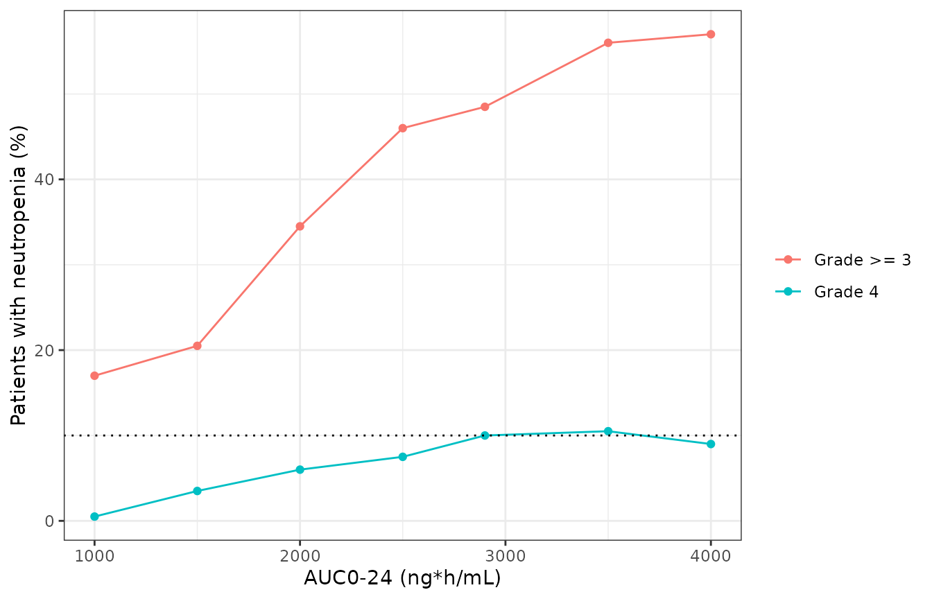
Replicates Figure 5 of Courlet 2022: incidence of grade >= 3 and grade 4 neutropenia over three cycles against AUC0-24 (200 patients per AUC value). Dotted line: the 10% threshold.
risk |>
  dplyr::rename("AUC0-24 (ng*h/mL)" = auc, "Grade >= 3 (%)" = g3, "Grade 4 (%)" = g4) |>
knitr::kable(digits = 1, caption = "Simulated neutropenia incidence by AUC0-24.")| AUC0-24 (ng*h/mL) | Grade >= 3 (%) | Grade 4 (%) |
|---|---|---|
| 1000 | 17.0 | 0.5 |
| 1500 | 20.5 | 3.5 |
| 2000 | 34.5 | 6.0 |
| 2500 | 46.0 | 7.5 |
| 2900 | 48.5 | 10.0 |
| 3500 | 56.0 | 10.5 |
| 4000 | 57.0 | 9.0 |
Progression-free survival (not encoded)
Section 3.3 and Supplementary Table S2 report a Cox proportional-hazards model for progression-free survival with AUCcum90 as a time-dependent covariate, older age (> 65 years) and their interaction. The coefficients are 0.030 per 100 ngh/mL of AUCcum90 (HR 1.030, p = 0.682), -0.872 for older age (HR 0.418, p = 0.048) and -0.125 per 100 ngh/mL for the interaction (HR 0.883, p = 0.266). A Cox model leaves the baseline hazard unspecified and the paper does not report it, so survival cannot be simulated and this sub-model is not packaged.
Assumptions and deviations
- Two final models. The paper reports a final PK-only model (Table S1) and a final PK/PD model in which the PK parameters were re-estimated together with the PD parameters (Table 2). Both are packaged. The fasting-plus-PPI clearance differs between them: 106 L/h (+56%, the value quoted in the Results and used for the Figure 3 simulation) in the PK-only model and 131 L/h (+96%) in the PK/PD model.
-
PPI and fasting covariate. The effect is coded as
the interaction
CONMED_PPI * (1 - FED), which switches clearance fromlclto the separately estimatedlcl_ppifasted.FED = 0covers fasting and a light meal, as in Section 3.2.1. The CL/F random effect applies in both states. -
Variance scale. Tables S1 and 2 report the IIV as
CV% with no stated formula. The CV% values are converted with
omega^2 = log(CV^2 + 1), as for the other Lausanne-group models in the library. The bootstrap percentile intervals cannot tell this apart fromomega^2 = (CV/100)^2. The two readings differ noticeably only for ka (125%) and EC50 (93%). -
Residual errors. The palbociclib error is
proportional (18%). The ANC error is additive on log-transformed ANC
(Section 2.3.2) and is encoded as log-normal (
lnorm) with SD 0.31. - Initial conditions. The paper does not state them. As in Friberg’s model, all five neutrophil compartments start at Base.
- Neutropenia simulations. The paper does not say whether residual error entered the incidence and nadir figures. Incidence is computed here on the individual ANC without residual error, and it matches the published values closely. The Figure 4 ribbons are likewise drawn without residual error.
- Recovery time. “Recovery to the base value” is read as the first time after the last dose at which ANC is back at or above the patient’s own baseline. The model gives a median of about 27 days, against 25 days in the paper. The paper says all simulated patients recovered; in the packaged model a small fraction (reported above) is still just below baseline 44 days after the last dose, because the feedback brings ANC back towards baseline asymptotically when the rebound does not overshoot.
- Covariates. Fulvestrant co-administration, prior chemotherapy and point-of-care ANC measurement were tested on the PD parameters and not retained (Section 3.2.2), so they are not model inputs.
- Literature check. No erratum or correction was found on Europe PMC or the journal page (checked 2026-10-03).