Tramadol enantiomers, metabolites and pain score in neuropathic pain (Chun 2025)
Source:vignettes/articles/Chun_2025_tramadol.Rmd
Chun_2025_tramadol.RmdModel and source
Chun 2025 built two enantiomer-specific population PK models for oral racemic tramadol in adults with chronic neuropathic pain, each describing total and unbound tramadol, total and unbound O-desmethyltramadol (M1) and unbound N-desmethyltramadol (M2). The (1R,2R) model also carries the pain-score PD model, which is driven by unbound (1R,2R)-M1, the mu-opioid agonist. The two enantiomers were fitted separately, so they are packaged as two model files:
Chun_2025_tramadol_rr: (1R,2R)-tramadol, M1, M2 and VAS pain score.Chun_2025_tramadol_ss: (1S,2S)-tramadol, M1 and M2.Citation: Chun D, Mehta P, Guzy S, Cicali B, Lauretti GR, Lanchote VL, Vozmediano V, De Moraes N. Enhanced Sensitivity to Tramadol in Diabetic Neuropathic Pain Compared to Nerve Compression Neuropathies: A Population PK/PD Model Analysis. CPT Pharmacometrics Syst Pharmacol. 2025;14(4):781-795. doi:10.1002/psp4.13315
Article: https://doi.org/10.1002/psp4.13315 (open access; the Supporting Information holds the NONMEM control streams, Tables S6 and S7, and the authors’ rxode2 simulation code, Table S8).
mod_rr <- readModelDb("Chun_2025_tramadol_rr")
mod_ss <- readModelDb("Chun_2025_tramadol_ss")
ui_rr <- rxode2::rxode2(mod_rr)
#> ℹ parameter labels from comments will be replaced by 'label()'
ui_ss <- rxode2::rxode2(mod_ss)
#> ℹ parameter labels from comments will be replaced by 'label()'
Structure
-
Tramadol: two-compartment disposition of the
unbound drug with a Weibull time-dependent absorption rate,
ka(t) = 1 - exp(-(ra * (t - tlag))^gam1)per hour (Equation 4;rais the reciprocal of the paper’s scalebeta,tlagits locationgamma). Unbound tramadol leaves the central compartment by M1 formation (fm_m1 * CLF,M1), an “other” route (0.3 * CLother) and Michaelis-Menten formation of M2. -
First pass: the oral dose is split. A fraction
1 - fpenters the tramadol depot andfp = FRAC / (1 + FRAC)enters a first-pass depot that delivers M1 directly at rateKmet1. Event tables must dose bothdepotanddepot_m1with the full enantiomer amount; the model’sf()splits it. -
M1: one compartment with biliary clearance into a
gallbladder that releases at
KrelbetweenSTARTTIMEandSTARTTIME + DURATIONafter the dose. The total M1 volume is scaled from the rat with an allometric exponent of 1 and divided byfu_M1to give the unbound volume. -
Protein binding: total = unbound / fu with
fu = 1 / (1 + Kb)(Equations 1-3), for tramadol and for M1. Diabetes (type 1 or type 2) multipliesKb. -
Pain score:
VAS = 100 * PD0 * (1 - Imax * Ce / (IC50 + Ce)), withCean effect compartment driven by unbound (1R,2R)-M1 (Equations 5 and 6), logit-normal IIV onImaxandPD0and an additive residual on the logit scale (Equations 7 and 8). Diabetes multipliesIC50.
Amounts are in nmol and concentrations in nmol/L of each enantiomer, as in the source. A 100 mg racemic dose is 50 mg of each enantiomer, 189,846 nmol with the 263.37 g/mol molar mass the paper uses.
mw_tramadol <- 263.37 # g/mol, Chun 2025 Methods
mw_metab <- 249.35 # g/mol, M1 and M2
nmol_per_mg <- 1e6 / mw_tramadol
Population
Thirty adults (16 women, 53%) aged 19-59 years with chronic neuropathic pain for more than 3 months, enrolled at the Hospital of the University of Sao Paulo, Brazil: 12 with neuropathic pain secondary to nerve compression (cervical or lumbar disc herniation, carpal tunnel syndrome), 9 with type 1 diabetes and 9 with type 2 diabetes (median HbA1c 10.7%). Mean BMI 27.3 kg/m^2 (range 17.2-38.9). Each received one 100 mg oral dose of racemic tramadol after an 8-hour fast; 2145 total and unbound concentrations of the tramadol, M1 and M2 enantiomers were collected over 24 h, and 402 VAS pain scores from 27 patients (three non-responders were excluded from the PD analysis). CYP2D6 activity was phenotyped as the metoprolol / alpha-hydroxymetoprolol ratio in 0-8 h urine (Chun 2025 Methods, Results “Data” and Table S2).
str(rxode2::rxode(mod_rr)$population[c("n_subjects", "age_range", "sex_female_pct", "regions")])
#> ℹ parameter labels from comments will be replaced by 'label()'
#> List of 4
#>  $ n_subjects    : int 30
#>  $ age_range     : chr "19-59 years"
#>  $ sex_female_pct: num 53.3
#>  $ regions       : chr "Brazil (Hospital of the University of Sao Paulo)"
Source trace
Every ini() value carries an in-file comment naming its
source. The table collects them; the (1S,2S) column is blank for the PD
parameters, which exist only in the (1R,2R) model.
| Parameter | (1R,2R) | (1S,2S) | Source |
|---|---|---|---|
Weibull shape gam1 (alpha) |
2.96 | 3.63 | Table 1 |
Weibull scale beta (h), ra = 1/beta
|
0.762 | 0.779 | Table 1 (row labels swapped; roles from Table S6/S7 code) |
Weibull location tlag (gamma, h) |
0.147 | 0.087 | Table 1 |
vc, Vc,u/F (L) |
63.4 | 78.1 | Table 1 |
e_bmi_vc, BMI power on Vc,u/F (ref 26.045 kg/m^2) |
3.87 | 3.43 | Table 1 beta1; Methods (reference) |
vp, Vp,u/F (L) |
439 | 465 | Table 1 |
q, Q,u/F (L/h) |
299 | 337 | Table 1 |
cl, CLother,u (L/h) |
36.4 | 38.6 | Table 1 |
fm_other (fixed) |
0.3 | 0.3 | Methods; Table S6/S7 (iii) |
kns, Kb of tramadol |
0.718 | 0.774 | Table 1 |
e_t1dm_kns, e_t2dm_kns
|
0.311, 0.95 | 0.15, 0.93 | Table 1 beta2, beta3 |
fm_m1 |
0.538 | 0.415 | Table 1 |
cl_form_m1, CLF,M1,u/F (L/h) |
58.8 | 159 | Table 1 |
e_cyp2d6_cl_form_m1 (ref ratio 0.610) |
-0.523 | -0.161 | Table 1 beta4; Methods |
fprat_m1, FRAC |
0.0661 | 0.0639 | Table 1 |
ka_m1, Kmet1 (1/h) |
0.796 | 1.51 | Table 1 |
vc_m1, total M1 volume (L, fixed) |
0.1 x 72.2/0.235 | 0.255 x 72.2/0.235 | Methods (rat scaling); Table S6/S7 |
cl_m1, CLM1,u/F (L/h) |
42 | 120 | Table 1 |
kns_m1, Kb of M1 |
3.07 | 3.65 | Table 1 |
e_t1dm_kns_m1, e_t2dm_kns_m1
|
0.105, 0.821 | 0.414, 0.467 | Table 1 beta5, beta6 |
cl_bile_m1, CLbile,u/F (L/h) |
382 | 406 | Table 1 |
kehc_m1, Krel,u (1/h) |
0.0019 | 0.039 | Table 1 |
tmeal1, STARTTIME (h) |
2.85 | 2.53 | Table 1 |
dge, DURATION (h) |
6.15 | 7.99 | Table 1 |
vmax_m2 (nmol/h) |
98.6 | 139 | Table 1 |
km_m2 (nmol, amount) |
16,300 | 21,500 | Table 1; Table S6/S7 (iii) code |
vc_m2, VM2,u/F (L) |
3.13 | 2.03 | Table 1 |
cl_m2, CLM2,u/F (L/h) |
7.75 | 13.4 | Table 1 |
e_cyp2d6_cl_m2 |
-0.477 | -0.401 | Table 1 beta7 |
ke0 (1/h) |
0.0398 | Table 1 | |
imax, e0 (PD0) |
0.908, 0.464 | Table 1 | |
ic50 (nmol/L); T1DM, T2DM factors |
2.36; 0.229, 0.431 | Table 1 beta8, beta9 | |
| IIV variances | Table 1 omega2 rows | Table 1 omega2 rows | Table 1; Table S8 |
| Residual variances | Table 1 sigma2 rows | Table 1 sigma2 rows | Table 1 |
| Parent ODEs, M1 ODEs with first pass and bile | Table S6/S7 (iii) $DES; Figure 1 |
||
| PD effect compartment and Imax model | Equations 5-8; Table S6 (iv) |
Deterministic checks
The fraction unbound of each species in a subject without diabetes,
and the derived first-pass fraction and the M2 fraction that the paper
back-calculates as fm2 = 1 - fm1 - fp - 0.3, follow from
the typical values alone.
typical_values <- function(ui) {
  th <- ui$theta
  fp <- exp(th[["lfprat_m1"]]) / (1 + exp(th[["lfprat_m1"]]))
  c(
    fu = 1 / (1 + exp(th[["lkns"]])),
    fu_m1 = 1 / (1 + exp(th[["lkns_m1"]])),
    fp = fp,
    fm_m2 = 1 - th[["fm_m1"]] - fp - th[["fm_other"]]
  )
}
chk <- rbind(
  "(1R,2R) model" = typical_values(ui_rr),
  "(1S,2S) model" = typical_values(ui_ss),
  "(1R,2R) paper" = c(0.582, 0.246, 0.062, 0.10),
  "(1S,2S) paper" = c(0.564, 0.215, 0.060, 0.225)
)
knitr::kable(chk, digits = 3, caption = "Typical-value fractions against Table 1 and Figure S19.")| fu | fu_m1 | fp | fm_m2 | |
|---|---|---|---|---|
| (1R,2R) model | 0.582 | 0.246 | 0.062 | 0.100 |
| (1S,2S) model | 0.564 | 0.215 | 0.060 | 0.225 |
| (1R,2R) paper | 0.582 | 0.246 | 0.062 | 0.100 |
| (1S,2S) paper | 0.564 | 0.215 | 0.060 | 0.225 |
Virtual cohort
Observed data are not available. Covariates are set to the cohort medians the paper uses for its own exposure comparisons (BMI 26.045 kg/m^2, metoprolol metabolic ratio 0.610) and the diabetes group is varied.
Between-subject random effects are drawn in base R from each model’s
omega matrix and passed as data columns, with the rxode2 random effects
switched off (omega = NA). The same 200 draws are reused in
every diabetes group and dosing regimen, so the comparisons below are
paired, and the cohort is identical on any machine and thread count.
draw_etas <- function(ui, n) {
  om <- ui$omega
  stopifnot(all(om[upper.tri(om)] == 0))
  sds <- sqrt(diag(om))
  as.data.frame(lapply(sds, function(s) stats::rnorm(n, 0, s)))
}

groups <- tibble(
  group = factor(c("No diabetes", "T1DM", "T2DM"), levels = c("No diabetes", "T1DM", "T2DM")),
  DIS_DIAB = c(0L, 1L, 1L),
  DIS_DIAB_TYPE2 = c(0L, 0L, 1L)
)

# Event table for one regimen: doses of the racemate (mg) at `dose_times`,
# each split equally between the enantiomers and given to BOTH depots.
make_events <- function(etas, dose_mg_rac, dose_times, obs_times, grp, id_offset = 0L) {
  n <- nrow(etas)
  amt <- dose_mg_rac / 2 * nmol_per_mg
  subj <- bind_cols(tibble(id = id_offset + seq_len(n)), etas)
  doses <- tidyr::expand_grid(id = subj$id, time = dose_times, cmt = c("depot", "depot_m1")) |>
    mutate(amt = amt, evid = 1L, dvid = NA_integer_)
  obs <- tidyr::expand_grid(id = subj$id, time = obs_times) |>
    mutate(cmt = "central", amt = 0, evid = 0L, dvid = 1L)
  bind_rows(doses, obs) |>
    left_join(subj, by = "id") |>
    mutate(
      BMI = 26.045, CYP2D6 = 0.610,
      DIS_DIAB = grp$DIS_DIAB, DIS_DIAB_TYPE2 = grp$DIS_DIAB_TYPE2,
      group = grp$group
    ) |>
    arrange(id, time, desc(evid))
}

solve_typical <- function(ui, events, keep = "group") {
  rxode2::rxSolve(ui, events,
    returnType = "data.frame", omega = NA, sigma = NA,
    useLinCmt = FALSE, keep = keep
  )
}

n_per_arm <- 200L
set.seed(20250213)
etas_rr <- draw_etas(ui_rr, n_per_arm)
etas_ss <- draw_etas(ui_ss, n_per_arm)
zero_eta <- function(etas) etas[1, , drop = FALSE] * 0
Typical single-dose profiles (Figure S1, Figure 2)
Typical-value profiles after 100 mg racemic tramadol in a subject without diabetes. Figure S1 of the paper shows the observed individual and mean concentrations; the observed means peak at roughly 70 ng/mL (unbound) and 120 ng/mL (total) for (1R,2R)-tramadol at 1.5-2 h and about 12 and 50 ng/mL for unbound and total (1R,2R)-M1.
grid <- sort(unique(c(seq(0, 4, by = 0.1), seq(4.5, 24, by = 0.5))))
typ <- bind_rows(
  solve_typical(ui_rr, make_events(zero_eta(etas_rr), 100, 0, grid, groups[1, ])) |>
    mutate(enantiomer = "(1R,2R)"),
  solve_typical(ui_ss, make_events(zero_eta(etas_ss), 100, 0, grid, groups[1, ])) |>
    mutate(enantiomer = "(1S,2S)")
) |>
  transmute(enantiomer, time,
    `Tramadol unbound` = Cunbound * mw_tramadol / 1000,
    `Tramadol total` = Cc * mw_tramadol / 1000,
    `M1 unbound` = Cunbound_m1 * mw_metab / 1000,
    `M1 total` = Cc_m1 * mw_metab / 1000,
    `M2 unbound` = Cc_m2 * mw_metab / 1000
  ) |>
  pivot_longer(-c(enantiomer, time), names_to = "analyte", values_to = "conc")

ggplot(typ, aes(time, conc, colour = enantiomer)) +
  geom_line() +
  facet_wrap(~analyte, scales = "free_y") +
  labs(x = "Time after dose (h)", y = "Concentration (ng/mL)", colour = NULL,
       caption = "Typical-value predictions, compare with Figure S1 / Figure S2 of Chun 2025.") +
  theme_bw() + theme(legend.position = "bottom")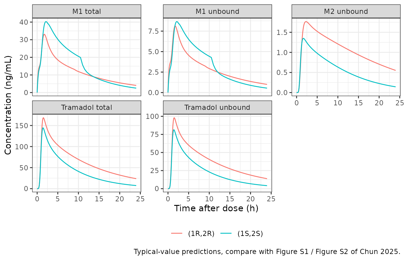
typ_peak <- typ |> group_by(enantiomer, analyte) |>
  summarise(Cmax = max(conc), tmax = time[which.max(conc)], .groups = "drop")
knitr::kable(typ_peak, digits = c(0, 0, 1, 2), caption = "Typical-value peaks (ng/mL, h).")| enantiomer | analyte | Cmax | tmax |
|---|---|---|---|
| (1R,2R) | M1 total | 33.1 | 1.7 |
| (1R,2R) | M1 unbound | 8.1 | 1.7 |
| (1R,2R) | M2 unbound | 1.8 | 2.3 |
| (1R,2R) | Tramadol total | 168.5 | 1.5 |
| (1R,2R) | Tramadol unbound | 98.1 | 1.5 |
| (1S,2S) | M1 total | 40.3 | 2.1 |
| (1S,2S) | M1 unbound | 8.7 | 2.1 |
| (1S,2S) | M2 unbound | 1.3 | 1.7 |
| (1S,2S) | Tramadol total | 144.5 | 1.4 |
| (1S,2S) | Tramadol unbound | 81.5 | 1.4 |
The typical (1R,2R)-tramadol peak sits close to the observed means. The typical M1 curves lie below the observed means of Figure S1; with a 0.73 variance on the formation clearance and 0.49 on the biliary clearance the mean of the observed profiles sits well above the typical curve. Total concentrations are unbound divided by fu at every time, which the model reproduces exactly:
Effect of diabetes on exposure (Figure 3) and fu (Figure 4)
The paper simulated 500 subjects per diabetes group after a 100 mg single dose with BMI and CYP2D6 activity at their medians and reported the ratio of median AUC0-24 and Cmax against subjects without diabetes. Here the same 200 paired subjects are solved in each group and exposures are computed with PKNCA.
grid_nca <- sort(unique(c(0, seq(0.25, 4, by = 0.25), seq(5, 24, by = 1))))
sim_dm <- bind_rows(lapply(seq_len(nrow(groups)), function(i) {
  solve_typical(ui_rr, make_events(etas_rr, 100, 0, grid_nca, groups[i, ], id_offset = (i - 1L) * n_per_arm))
}))
dose_dm <- bind_rows(lapply(seq_len(nrow(groups)), function(i) {
  make_events(etas_rr, 100, 0, grid_nca, groups[i, ], id_offset = (i - 1L) * n_per_arm)
})) |>
  filter(evid == 1, cmt == "depot") |>
  select(id, time, amt, group)
nca_one <- function(sim, conc_col, label) {
  conc <- sim |>
    transmute(id, time, group, conc = .data[[conc_col]]) |>
    filter(!is.na(conc))
  conc <- bind_rows(conc, conc |> distinct(id, group) |> mutate(time = 0, conc = 0)) |>
    distinct(id, group, time, .keep_all = TRUE) |>
    arrange(id, time)
  conc_obj <- PKNCA::PKNCAconc(conc, conc ~ time | group + id)
  dose_obj <- PKNCA::PKNCAdose(dose_dm, amt ~ time | group + id)
  intervals <- data.frame(start = 0, end = 24, cmax = TRUE, auclast = TRUE)
  res <- PKNCA::pk.nca(PKNCA::PKNCAdata(conc_obj, dose_obj, intervals = intervals))
  as.data.frame(res) |> mutate(analyte = label)
}
nca_dm <- bind_rows(
  nca_one(sim_dm, "Cunbound", "Tramadol unbound"),
  nca_one(sim_dm, "Cc", "Tramadol total"),
  nca_one(sim_dm, "Cunbound_m1", "M1 unbound"),
  nca_one(sim_dm, "Cc_m1", "M1 total")
)
ratios <- nca_dm |>
  group_by(analyte, PPTESTCD, group) |>
  summarise(med = median(PPORRES), .groups = "drop") |>
  group_by(analyte, PPTESTCD) |>
  mutate(ratio = med / med[group == "No diabetes"]) |>
  ungroup() |>
  filter(group != "No diabetes")

ratios |>
  select(analyte, PPTESTCD, group, ratio) |>
  pivot_wider(names_from = group, values_from = ratio) |>
  rename(Analyte = analyte, `NCA parameter` = PPTESTCD) |>
knitr::kable(digits = 2, caption = "Ratio of median exposure against subjects without diabetes (Figure 3).")| Analyte | NCA parameter | T1DM | T2DM |
|---|---|---|---|
| M1 total | auclast | 0.30 | 0.85 |
| M1 total | cmax | 0.35 | 0.89 |
| M1 unbound | auclast | 1.00 | 1.00 |
| M1 unbound | cmax | 1.09 | 1.03 |
| Tramadol total | auclast | 0.72 | 0.99 |
| Tramadol total | cmax | 0.72 | 0.98 |
| Tramadol unbound | auclast | 1.00 | 1.00 |
| Tramadol unbound | cmax | 1.00 | 1.00 |
ggplot(ratios, aes(ratio, analyte, colour = group)) +
  annotate("rect", xmin = 0.8, xmax = 1.25, ymin = -Inf, ymax = Inf, alpha = 0.15) +
  geom_point(size = 2.5, position = position_dodge(width = 0.5)) +
  geom_vline(xintercept = 1, linetype = 2) +
  facet_wrap(~PPTESTCD) +
  labs(x = "Ratio of median vs no diabetes", y = NULL, colour = NULL,
       caption = "Replicates Figure 3 of Chun 2025 (100 mg single dose, covariates at median).") +
  theme_bw() + theme(legend.position = "bottom")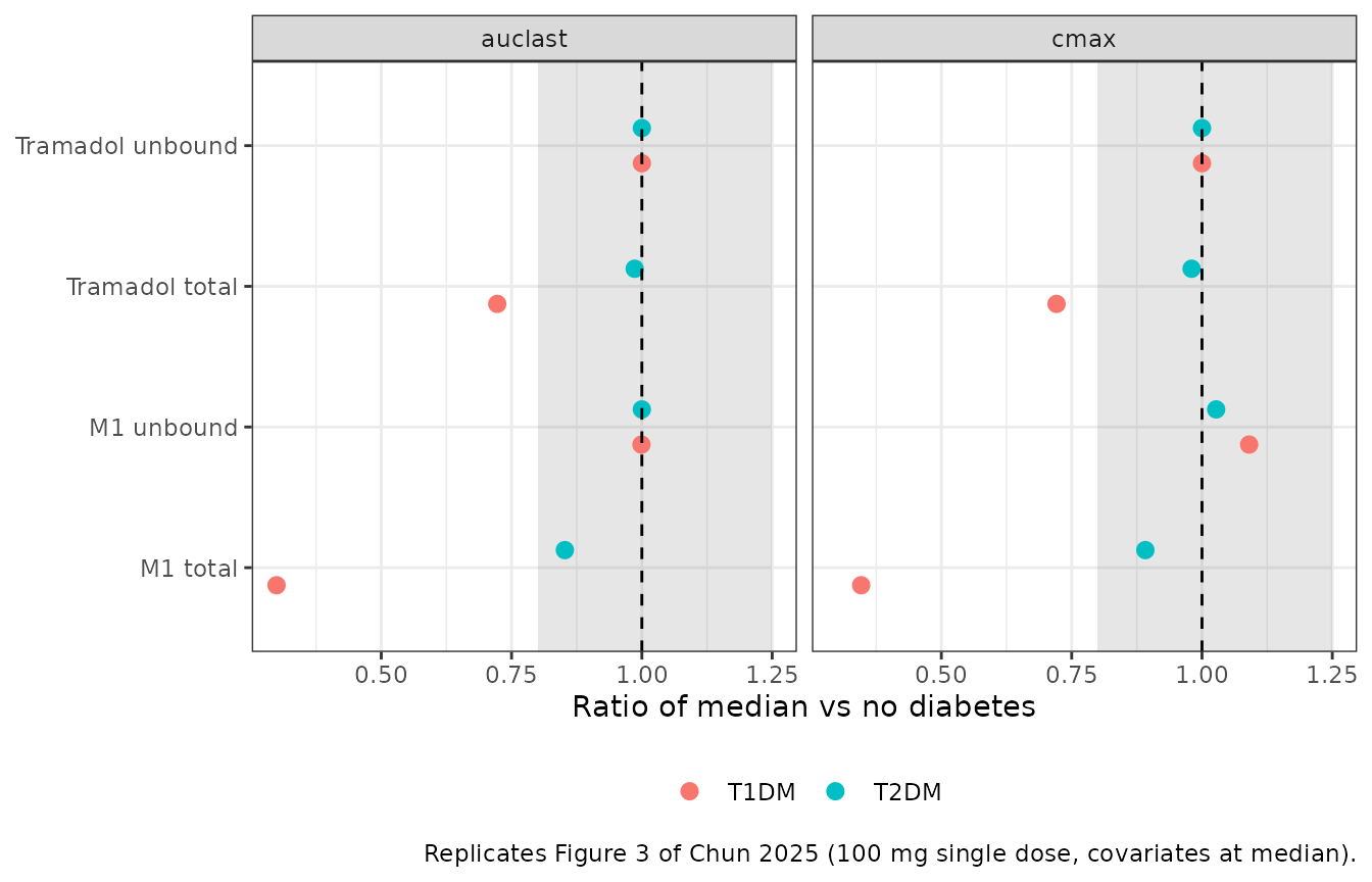
The paper reports a 67% (type 1) and 14% (type 2) lower AUC of total (1R,2R)-M1 and an unchanged unbound (1R,2R)-M1 AUC. Diabetes changes only the binding constants, so the unbound M1 AUC moves little and the total M1 AUC follows the change in fu.
r_auc <- function(an, grp) {
  v <- ratios$ratio[ratios$analyte == an & ratios$PPTESTCD == "auclast" & ratios$group == grp]
  if (length(v) != 1L) stop("no unique ratio for ", an, " / ", grp)
  v
}
stopifnot(
  abs(r_auc("M1 total", "T1DM") - (1 - 0.67)) < 0.08,
  abs(r_auc("M1 total", "T2DM") - (1 - 0.14)) < 0.08,
  abs(r_auc("M1 unbound", "T1DM") - 1) < 0.15,
  abs(r_auc("M1 unbound", "T2DM") - 1) < 0.15
)
fu_tab <- bind_rows(
  sim_dm |> distinct(id, group, fu, fu_m1) |> mutate(enantiomer = "(1R,2R)"),
  bind_rows(lapply(seq_len(nrow(groups)), function(i) {
    solve_typical(ui_ss, make_events(etas_ss, 100, 0, 1, groups[i, ], id_offset = (i - 1L) * n_per_arm))
  })) |> distinct(id, group, fu, fu_m1) |> mutate(enantiomer = "(1S,2S)")
) |>
  pivot_longer(c(fu, fu_m1), names_to = "species", values_to = "fu") |>
  mutate(species = ifelse(species == "fu", "Tramadol", "M1"))

ggplot(fu_tab, aes(group, fu, fill = group)) +
  geom_boxplot(outlier.size = 0.5) +
  facet_grid(enantiomer ~ species) +
  labs(x = NULL, y = "Fraction unbound", fill = NULL,
       caption = "Replicates Figure 4 of Chun 2025 (simulated fu by diabetes group).") +
  theme_bw() + theme(legend.position = "none")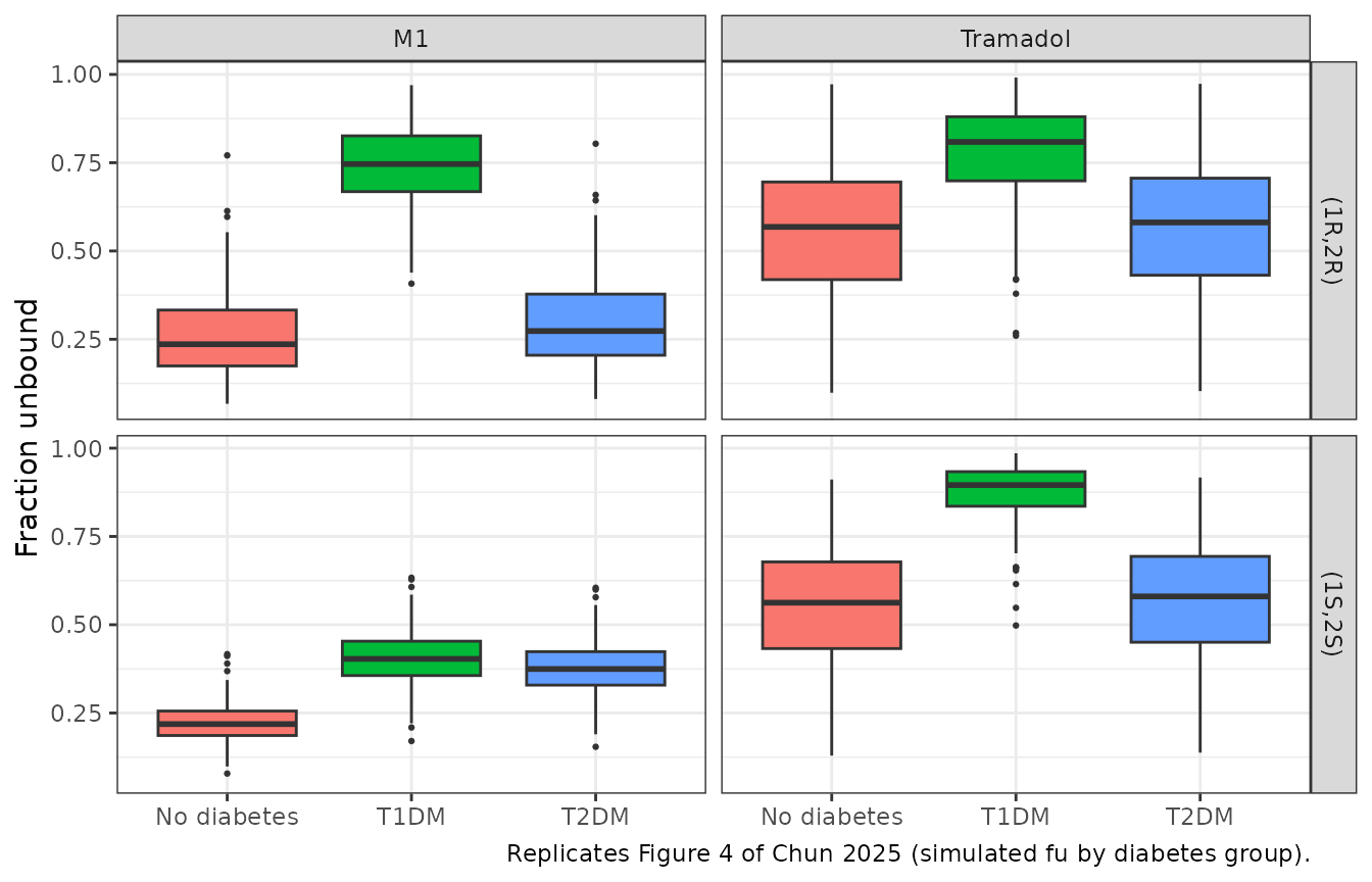
fu_tab |> group_by(enantiomer, species, group) |>
  summarise(`median fu` = median(fu), .groups = "drop") |>
  pivot_wider(names_from = group, values_from = `median fu`) |>
knitr::kable(digits = 3, caption = "Median simulated fraction unbound.")| enantiomer | species | No diabetes | T1DM | T2DM |
|---|---|---|---|---|
| (1R,2R) | M1 | 0.236 | 0.746 | 0.273 |
| (1R,2R) | Tramadol | 0.568 | 0.809 | 0.581 |
| (1S,2S) | M1 | 0.219 | 0.403 | 0.375 |
| (1S,2S) | Tramadol | 0.562 | 0.895 | 0.580 |
Pain relief by dosing regimen (Table 2, Figure 5)
Table 2 reports the percentage of 500 simulated subjects per group
with substantial (> 50% below baseline) or moderate (30-50%) pain
relief, at the time of maximum relief after a single dose and at the
trough 72 h into repeated dosing. Pain is normalised by each subject’s
baseline, so the residual error and PD0 drop out and relief
is Imax * Ce / (IC50 + Ce).
The authors’ simulation code (Table S8) evaluates that expression on
the plasma unbound M1 concentration rather than on the
effect-compartment concentration of the fitted PD model (Equations 5 and
6). Both are computed below: relief_effect uses the
packaged model’s effect compartment and relief_plasma
mirrors Table S8.
regimens <- tribble(
  ~regimen, ~dose, ~tau,
  "50 mg q.d.", 50, 24,
  "100 mg q.d.", 100, 24,
  "200 mg q.d.", 200, 24,
  "400 mg q.d.", 400, 24,
  "50 mg b.i.d.", 50, 12,
  "100 mg b.i.d.", 100, 12,
  "200 mg b.i.d.", 200, 12
)
obs72 <- seq(0, 72, by = 1)
pd_events <- bind_rows(lapply(seq_len(nrow(regimens)), function(r) {
  bind_rows(lapply(seq_len(nrow(groups)), function(i) {
    k <- (r - 1L) * nrow(groups) + i
    make_events(etas_rr, regimens$dose[r], seq(0, 72 - regimens$tau[r], by = regimens$tau[r]),
      obs72, groups[i, ], id_offset = (k - 1L) * n_per_arm) |>
      mutate(regimen = regimens$regimen[r])
  }))
}))
sim_pd <- solve_typical(ui_rr, pd_events, keep = c("group", "regimen")) |>
  mutate(
    relief_effect = imax * effect / (ic50 + effect),
    relief_plasma = imax * Cunbound_m1 / (ic50 + Cunbound_m1),
    regimen = factor(regimen, levels = regimens$regimen)
  )
classify <- function(x) {
  c(substantial = 100 * mean(x > 0.5), moderate = 100 * mean(x >= 0.3 & x <= 0.5))
}
relief_summary <- function(sim, col) {
  max_sd <- sim |> filter(time <= 24) |> group_by(regimen, group, id) |>
    summarise(r = max(.data[[col]]), .groups = "drop")
  trough <- sim |> filter(time == 72) |> group_by(regimen, group, id) |>
    summarise(r = .data[[col]][1], .groups = "drop")
  bind_rows(
    max_sd |> mutate(when = "Maximum"),
    trough |> mutate(when = "Sustained")
  ) |>
    group_by(regimen, group, when) |>
    summarise(substantial = classify(r)[["substantial"]], moderate = classify(r)[["moderate"]], .groups = "drop")
}
tab_plasma <- relief_summary(sim_pd, "relief_plasma") |> mutate(driver = "plasma (Table S8)")
tab_effect <- relief_summary(sim_pd, "relief_effect") |> mutate(driver = "effect compartment (model)")

published_t2 <- tribble(
  ~regimen, ~group, ~when, ~substantial, ~moderate,
  "50 mg q.d.", "No diabetes", "Sustained", 22.4, 29.6,
  "50 mg q.d.", "T1DM", "Sustained", 61.0, 17.0,
  "50 mg q.d.", "T2DM", "Sustained", 51.0, 22.4,
  "100 mg q.d.", "No diabetes", "Sustained", 43.0, 23.0,
  "100 mg q.d.", "T1DM", "Sustained", 70.4, 11.6,
  "100 mg q.d.", "T2DM", "Sustained", 65.0, 15.6,
  "200 mg q.d.", "No diabetes", "Sustained", 59.0, 17.4,
  "200 mg q.d.", "T1DM", "Sustained", 75.4, 8.4,
  "200 mg q.d.", "T2DM", "Sustained", 74.8, 9.2,
  "400 mg q.d.", "No diabetes", "Sustained", 67.2, 13.6,
  "400 mg q.d.", "T1DM", "Sustained", 76.4, 7.8,
  "400 mg q.d.", "T2DM", "Sustained", 78.4, 7.6,
  "50 mg b.i.d.", "No diabetes", "Sustained", 61.2, 17.4,
  "50 mg b.i.d.", "T1DM", "Sustained", 76.0, 8.6,
  "50 mg b.i.d.", "T2DM", "Sustained", 77.4, 9.4,
  "100 mg b.i.d.", "No diabetes", "Sustained", 70.8, 12.2,
  "100 mg b.i.d.", "T1DM", "Sustained", 77.2, 7.6,
  "100 mg b.i.d.", "T2DM", "Sustained", 81.2, 6.4,
  "200 mg b.i.d.", "No diabetes", "Sustained", 73.4, 11.0,
  "200 mg b.i.d.", "T1DM", "Sustained", 77.6, 7.8,
  "200 mg b.i.d.", "T2DM", "Sustained", 81.8, 6.2,
  "50 mg q.d.", "No diabetes", "Maximum", 72.0, 12.6,
  "50 mg q.d.", "T1DM", "Maximum", 78.2, 7.2,
  "50 mg q.d.", "T2DM", "Maximum", 81.8, 6.2,
  "100 mg q.d.", "No diabetes", "Maximum", 74.6, 10.4,
  "100 mg q.d.", "T1DM", "Maximum", 78.4, 7.0,
  "100 mg q.d.", "T2DM", "Maximum", 82.6, 5.4,
  "200 mg q.d.", "No diabetes", "Maximum", 75.0, 10.4,
  "200 mg q.d.", "T1DM", "Maximum", 78.6, 7.0,
  "200 mg q.d.", "T2DM", "Maximum", 82.8, 5.2,
  "400 mg q.d.", "No diabetes", "Maximum", 75.6, 9.8,
  "400 mg q.d.", "T1DM", "Maximum", 78.6, 7.0,
  "400 mg q.d.", "T2DM", "Maximum", 83.0, 5.0
)

cmp_t2 <- published_t2 |>
  inner_join(tab_plasma |> mutate(group = as.character(group), regimen = as.character(regimen)),
    by = c("regimen", "group", "when"), suffix = c("_paper", "_plasma")) |>
  inner_join(tab_effect |> mutate(group = as.character(group), regimen = as.character(regimen)) |>
    select(regimen, group, when, substantial_effect = substantial),
    by = c("regimen", "group", "when"))
stopifnot(nrow(cmp_t2) == nrow(published_t2))

cmp_t2 |>
  transmute(when, regimen, group,
    paper = sprintf("%.1f/%.1f", substantial_paper, moderate_paper),
    plasma = sprintf("%.1f/%.1f", substantial_plasma, moderate_plasma),
    effect = sprintf("%.1f", substantial_effect)
  ) |>
  rename(`Relief at` = when, Regimen = regimen, Group = group,
    `Paper (substantial/moderate %)` = paper,
    `Plasma-driven (substantial/moderate %)` = plasma,
    `Effect compartment (substantial %)` = effect) |>
knitr::kable(caption = "Table 2 of Chun 2025 against the packaged (1R,2R) model.")| Relief at | Regimen | Group | Paper (substantial/moderate %) | Plasma-driven (substantial/moderate %) | Effect compartment (substantial %) |
|---|---|---|---|---|---|
| Sustained | 50 mg q.d. | No diabetes | 22.4/29.6 | 22.5/32.0 | 61.5 |
| Sustained | 50 mg q.d. | T1DM | 61.0/17.0 | 59.0/16.5 | 73.5 |
| Sustained | 50 mg q.d. | T2DM | 51.0/22.4 | 49.5/19.0 | 69.5 |
| Sustained | 100 mg q.d. | No diabetes | 43.0/23.0 | 47.0/19.5 | 67.5 |
| Sustained | 100 mg q.d. | T1DM | 70.4/11.6 | 67.5/11.5 | 74.0 |
| Sustained | 100 mg q.d. | T2DM | 65.0/15.6 | 59.5/16.5 | 74.0 |
| Sustained | 200 mg q.d. | No diabetes | 59.0/17.4 | 57.5/18.0 | 73.5 |
| Sustained | 200 mg q.d. | T1DM | 75.4/8.4 | 70.0/12.0 | 74.5 |
| Sustained | 200 mg q.d. | T2DM | 74.8/9.2 | 68.0/11.5 | 74.0 |
| Sustained | 400 mg q.d. | No diabetes | 67.2/13.6 | 67.5/11.5 | 74.0 |
| Sustained | 400 mg q.d. | T1DM | 76.4/7.8 | 73.5/11.5 | 77.0 |
| Sustained | 400 mg q.d. | T2DM | 78.4/7.6 | 71.0/11.5 | 74.5 |
| Sustained | 50 mg b.i.d. | No diabetes | 61.2/17.4 | 64.0/13.5 | 69.0 |
| Sustained | 50 mg b.i.d. | T1DM | 76.0/8.6 | 73.5/10.5 | 74.0 |
| Sustained | 50 mg b.i.d. | T2DM | 77.4/9.4 | 71.5/10.0 | 74.0 |
| Sustained | 100 mg b.i.d. | No diabetes | 70.8/12.2 | 70.5/10.5 | 74.0 |
| Sustained | 100 mg b.i.d. | T1DM | 77.2/7.6 | 74.5/10.5 | 75.0 |
| Sustained | 100 mg b.i.d. | T2DM | 81.2/6.4 | 73.5/10.5 | 74.0 |
| Sustained | 200 mg b.i.d. | No diabetes | 73.4/11.0 | 73.5/10.0 | 74.0 |
| Sustained | 200 mg b.i.d. | T1DM | 77.6/7.8 | 75.5/10.0 | 77.0 |
| Sustained | 200 mg b.i.d. | T2DM | 81.8/6.2 | 74.5/11.0 | 75.5 |
| Maximum | 50 mg q.d. | No diabetes | 72.0/12.6 | 69.5/11.5 | 42.5 |
| Maximum | 50 mg q.d. | T1DM | 78.2/7.2 | 75.0/10.0 | 70.5 |
| Maximum | 50 mg q.d. | T2DM | 81.8/6.2 | 74.0/10.0 | 64.0 |
| Maximum | 100 mg q.d. | No diabetes | 74.6/10.4 | 73.5/8.5 | 60.5 |
| Maximum | 100 mg q.d. | T1DM | 78.4/7.0 | 75.5/10.0 | 74.0 |
| Maximum | 100 mg q.d. | T2DM | 82.6/5.4 | 75.0/10.0 | 71.0 |
| Maximum | 200 mg q.d. | No diabetes | 75.0/10.4 | 74.5/10.0 | 70.0 |
| Maximum | 200 mg q.d. | T1DM | 78.6/7.0 | 76.5/9.0 | 74.0 |
| Maximum | 200 mg q.d. | T2DM | 82.8/5.2 | 75.5/10.0 | 74.0 |
| Maximum | 400 mg q.d. | No diabetes | 75.6/9.8 | 75.5/10.0 | 74.0 |
| Maximum | 400 mg q.d. | T1DM | 78.6/7.0 | 77.5/8.0 | 75.0 |
| Maximum | 400 mg q.d. | T2DM | 83.0/5.0 | 76.5/9.0 | 74.0 |
d_sub <- cmp_t2$substantial_plasma - cmp_t2$substantial_paper
# The fraction above 50% relief is dominated by the logit-normal Imax
# distribution (variance 8.97); a mis-transcribed IC50, ke0 or Imax moves
# these percentages by tens of points.
stopifnot(
  abs(median(d_sub)) < 6,
  quantile(abs(d_sub), 0.9) < 15
)
With the plasma driver the packaged model tracks Table 2. The ranking
the paper draws from it holds: subjects with diabetes respond to lower
doses, and subjects with compression neuropathy gain more from
twice-daily than from once-daily dosing. Driving the response through
the effect compartment, as the fitted PD model does, keeps relief high
at trough because ke0 = 0.04 1/h gives the effect site a 17
h equilibration half-life.
sim_pd |>
  filter(regimen %in% c("50 mg q.d.", "100 mg q.d.", "200 mg q.d.", "400 mg q.d.",
                        "50 mg b.i.d.", "100 mg b.i.d.", "200 mg b.i.d.")) |>
  mutate(freq = ifelse(grepl("b.i.d", regimen), "b.i.d.", "q.d."),
         dose = sub(" mg.*", " mg", regimen)) |>
  group_by(time, group, freq, dose) |>
  summarise(pain = median(1 - relief_plasma), .groups = "drop") |>
  ggplot(aes(time, pain, colour = dose)) +
  geom_line() +
  facet_grid(freq ~ group) +
  labs(x = "Time (h)", y = "Median pain score / baseline", colour = "Dose",
       caption = "Replicates Figure 5 of Chun 2025 (plasma-driven response, as in Table S8).") +
  theme_bw() + theme(legend.position = "bottom")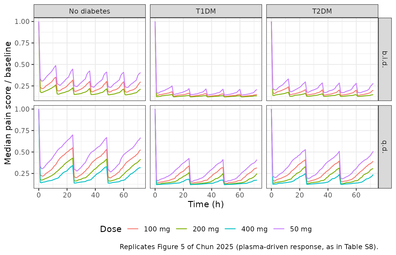
Multiple dosing (Figure S18)
Figure S18 compares the final model with the mean total tramadol and M1 concentrations of Karhu 2010 after 50 mg immediate-release racemic tramadol every 6 hours. Both enantiomer models are summed. The paper’s simulated mean reaches about 140 ng/mL after the first dose and about 320 ng/mL after the fourth dose for total tramadol, and about 40 and 80 ng/mL for total M1.
grid48 <- sort(unique(c(seq(0, 24, by = 0.25), seq(25, 48, by = 1))))
s18 <- function(ui, etas) {
  solve_typical(ui, make_events(etas, 50, c(0, 6, 12, 18), grid48, groups[1, ])) |>
    select(id, time, Cc, Cc_m1)
}
sum18 <- inner_join(s18(ui_rr, etas_rr), s18(ui_ss, etas_ss), by = c("id", "time"), suffix = c("_rr", "_ss")) |>
  transmute(id, time,
    tramadol = (Cc_rr + Cc_ss) * mw_tramadol / 1000,
    M1 = (Cc_m1_rr + Cc_m1_ss) * mw_metab / 1000
  ) |>
  pivot_longer(c(tramadol, M1), names_to = "analyte", values_to = "conc") |>
  group_by(analyte, time) |>
  summarise(mean = mean(conc), q05 = quantile(conc, 0.05), q95 = quantile(conc, 0.95), .groups = "drop")

ggplot(sum18, aes(time, mean)) +
  geom_ribbon(aes(ymin = q05, ymax = q95), alpha = 0.2) +
  geom_line() +
  facet_wrap(~analyte, scales = "free_y") +
  labs(x = "Time (h)", y = "Total racemic concentration (ng/mL)",
       caption = "Replicates the simulated curves of Figure S18 of Chun 2025 (50 mg every 6 h, no diabetes).") +
  theme_bw()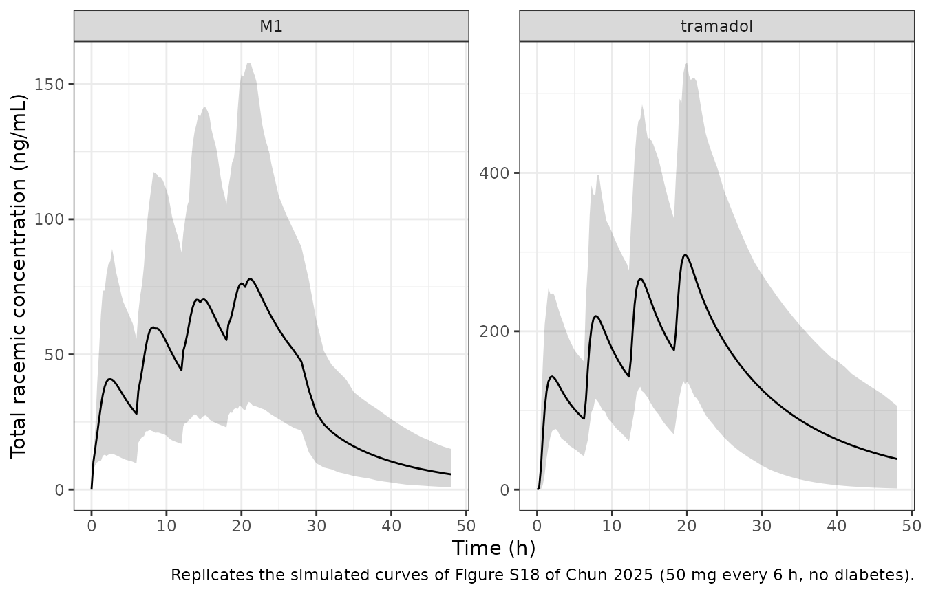
peaks18 <- sum18 |> filter(time <= 24) |>
  mutate(dose = cut(time, c(0, 6, 12, 18, 24), labels = paste("dose", 1:4), include.lowest = TRUE)) |>
  group_by(analyte, dose) |>
  summarise(peak = max(mean), .groups = "drop") |>
  mutate(figure_s18 = case_when(
    analyte == "tramadol" & dose == "dose 1" ~ 140,
    analyte == "tramadol" & dose == "dose 4" ~ 320,
    analyte == "M1" & dose == "dose 1" ~ 38,
    analyte == "M1" & dose == "dose 4" ~ 80
  ))
peaks18 |>
  rename(Analyte = analyte, Dose = dose, `Simulated peak mean (ng/mL)` = peak,
         `Figure S18, read from the plot (ng/mL)` = figure_s18) |>
knitr::kable(digits = 0)| Analyte | Dose | Simulated peak mean (ng/mL) | Figure S18, read from the plot (ng/mL) |
|---|---|---|---|
| M1 | dose 1 | 41 | 38 |
| M1 | dose 2 | 60 | NA |
| M1 | dose 3 | 70 | NA |
| M1 | dose 4 | 78 | 80 |
| tramadol | dose 1 | 143 | 140 |
| tramadol | dose 2 | 219 | NA |
| tramadol | dose 3 | 266 | NA |
| tramadol | dose 4 | 297 | 320 |
# The Figure S18 values are read off the plotted curve to about 5%. The
# M1 peaks in particular separate the fraction-of-dose reading of the
# first-pass split from the alternatives discussed under Assumptions.
chk18 <- peaks18 |> filter(!is.na(figure_s18))
stopifnot(nrow(chk18) == 4L, all(abs(log(chk18$peak / chk18$figure_s18)) < 0.2))
The summed enantiomer models reproduce the published simulated means of Figure S18 for both tramadol and M1 at the first and the fourth dose.
Assumptions and deviations
-
Two dosing records per dose. The dose is split
between the tramadol depot (
1 - fp) and the first-pass depot (fp) byf(), as described in Figure 1, Table 1 and the mass balance of Figure S19 and as implied by the authors’ simulation code (Table S8), whose depot outflows are not scaled. The NONMEM$DESblocks (Tables S6 and S7) instead multiply the two depot outflow rates by1 - fpandfp; how the estimation dataset apportioned the amounts between the two depots is not reported. The fraction-of-dose reading is the one that reproduces the published 6% first-pass share and the simulated M1 means of Figure S18; dosing both depots in full with the scaled outflows roughly doubles the total amount reaching the body and, in the maintainers’ check, raised the mean total (1R,2R)-M1 concentration at 3 h by about 80%. - Time after dose. The Weibull absorption rate and the gallbladder release window are read against the time after the most recent dose. The source data are single-dose, where this equals time since the dose; the authors’ own simulation code uses time since the start of the simulation, so later doses there are absorbed at the plateau rate of 1 per hour from the moment they are given.
-
Weibull parameter labels. Table 1 labels gamma
“scale” and beta “location”; the NONMEM code uses gamma as the location
(lag) and beta as the scale, and the model follows the code. The IIV on
beta is carried on its reciprocal
ra, which has the same variance. - IIV on the central volume. Table 1 labels the 1.29 / 1.09 variance and the BMI exponent as applying to Vp; the NONMEM code, Table S3 and the Results text place both on the central volume.
-
Michaelis-Menten constant of M2. Table 1 prints
Kmin nmol/L, but the NONMEM and rxode2 code divide by the central amount;km_m2is in nmol. - IC50 values in the text. The Results text quotes IC50 = 2.91 nmol/L (no diabetes), 0.156 (T1DM) and 0.515 nmol/L (T2DM). Table 1 and the code give 2.36 nmol/L with multipliers 0.229 and 0.431 (0.54 and 1.02 nmol/L); the model uses Table 1.
- (1S,2S) code differences. The authors’ simulation code for (1S,2S) uses Kmet1 = 1.59 1/h and the (1R,2R) BMI exponent 3.87, and for (1R,2R) CLM1,u/F = 47.7 L/h; the model uses the Table 1 values (1.51, 3.43 and 42).
-
Pain-score scale. The paper fits the VAS divided by
100. The model reports
scorein mm (0-100) with the same logit-scale residual,logitNorm(addSd_score, 0, 100). - Dose amount. The paper does not say whether the 100 mg Tramal dose was converted to moles as the base or as the hydrochloride; this vignette converts 50 mg per enantiomer with the 263.37 g/mol base molar mass, which reproduces the observed peak of (1R,2R)-tramadol.
- Covariates in the simulations. BMI and the metoprolol metabolic ratio are held at their medians, as the paper states for Figure 3; the paper does not state the covariates used for Table 2 and Figure S18.