Factor VIII (Allard 2020)
Source:vignettes/articles/Allard_2020_factorviii.Rmd
Allard_2020_factorviii.RmdModel and source
- Citation: Allard Q, Djerada Z, Pouplard C, Repesse Y, Desprez D, Galinat H, Frotscher B, Berger C, Harroche A, Ryman A, Flaujac C, Chamouni P, Guillet B, Volot F, Szymezak J, Nguyen P, Cazaubon Y. Real Life Population Pharmacokinetics Modelling of Eight Factors VIII in Patients with Severe Haemophilia A: Is It Always Relevant to Switch to an Extended Half-Life? Pharmaceutics. 2020;12(4):380. doi:10.3390/pharmaceutics12040380
- Description: Two-compartment population PK model for factor VIII activity (FVIII:C, one-stage clotting assay) pooled across eight standard and extended half-life FVIII concentrates in children, adolescents and adults with mainly severe haemophilia A (Allard 2020; weight and age on CL, weight on V1, Elocta (rFVIIIFc) indicator on CL)
- Article (open access): https://doi.org/10.3390/pharmaceutics12040380
Allard and colleagues pooled routine-care FVIII:C (one-stage clotting assay) measurements after eight FVIII concentrates – seven standard half-life (SHL) products and one extended half-life (EHL) product, Elocta (efmoroctocog alfa, rFVIIIFc) – into a single Monolix population PK model. The final model is a linear two-compartment model with power effects of weight and age on clearance, weight on the central volume, and an Elocta indicator on clearance.
Population
The analysis included 258 patients from 13 French haemophilia treatment centres (87 children and adolescents, 171 adults; Allard 2020 Table 1): median age 30 years (3-77), median weight 64 kg (15.1-130). Haemophilia was severe in 244 patients, moderate in 11 and minor in 3; none had inhibitors. PK profiles were recorded after Elocta (n = 136), Advate (44), Kogenate (34), Refacto (18), Factane (8), Kovaltry (7), Novoeight (6) and Afstyla (5); 44 patients switched from an SHL product to Elocta and contributed a profile on each. The 935 FVIII:C samples (1-11 per patient, median 4) were taken before and 15 min to 96 h after an intravenous dose of median 2750 IU (500-5000 IU); 10.6% were below the LLOQ. Sex is not reported.
The same information is available programmatically via
readModelDb("Allard_2020_factorviii")()$population.
Source trace
| Equation / parameter | Value | Source location |
|---|---|---|
lcl |
log(204 mL/h) | Table 2, Cl |
lvc |
log(2640 mL) | Table 2, V1 |
lq |
log(135 mL/h) | Table 2, Q |
lvp |
log(339 mL) | Table 2, V2 |
e_wt_cl |
0.75 (fixed) | Table 2, beta Weight on Cl ‘0.75 FIX’; Section 3.3 |
e_age_cl |
-0.214 | Table 2, beta Age; sign from the Table 2 footnote equation |
e_form_fviii_fc_cl |
-0.394 | Table 2, beta EHL; sign from the Table 2 footnote equation |
e_wt_vc |
0.827 | Table 2, beta Weight on V1 |
etalcl variance |
0.349^2 = 0.121801 | Table 2, omega Cl 34.9% |
etalvc variance |
0.232^2 = 0.053824 | Table 2, omega V1 23.2% |
cov(etalcl, etalvc) |
0.599 x 0.349 x 0.232 = 0.048500 | Table 2, Corr(V1, Cl) |
etalvp variance |
0.468^2 = 0.219024 | Table 2, omega V2 46.8% |
addSd |
0.00868 IU/mL | Table 2, a (constant) |
propSd |
0.108 | Table 2, b (proportional) 10.8% |
| Continuous covariate model | (COV / median)^beta |
Eq. 1; medians 30 years and 64 kg from the Table 2 footnote |
| Categorical covariate model | exp(beta * EHL) |
Eq. 2 |
| Residual error | y = Cc + (a + b * Cc) * e |
Eq. 3 (Monolix combined1) |
| Two-compartment linear ODEs | n/a | Section 3.2 |
Closed-form checks of the typical patient
The terminal half-life of a two-compartment model follows from its micro-constants. For the typical patient (30 years, 64 kg) the model gives:
mod <- readModelDb("Allard_2020_factorviii")
ini_est <- rxode2::rxode2(mod)$theta
#> ℹ parameter labels from comments will be replaced by 'label()'

half_life_2cmt <- function(cl, vc, q, vp) {
  k10 <- cl / vc
  k12 <- q / vc
  k21 <- q / vp
  s <- k10 + k12 + k21
  beta <- (s - sqrt(s^2 - 4 * k10 * k21)) / 2
  log(2) / beta
}

cl_shl <- exp(ini_est[["lcl"]])
cl_ehl <- exp(ini_est[["lcl"]] + ini_est[["e_form_fviii_fc_cl"]])
vc_typ <- exp(ini_est[["lvc"]])
q_typ <- exp(ini_est[["lq"]])
vp_typ <- exp(ini_est[["lvp"]])

typical <- tibble(
  product = c("Standard half-life", "Elocta"),
  `CL (mL/h)` = c(cl_shl, cl_ehl),
  `Terminal t1/2 (h)` = c(
    half_life_2cmt(cl_shl, vc_typ, q_typ, vp_typ),
    half_life_2cmt(cl_ehl, vc_typ, q_typ, vp_typ)
  )
)
knitr::kable(typical, digits = 2)| product | CL (mL/h) | Terminal t1/2 (h) |
|---|---|---|
| Standard half-life | 204.00 | 10.35 |
| Elocta | 137.57 | 15.23 |
hl_ratio_typ <- typical$`Terminal t1/2 (h)`[2] / typical$`Terminal t1/2 (h)`[1]
hl_ratio_typ
#> [1] 1.470854
The paper reports that half-life increased on average by a factor of
1.48 when patients switched from an SHL product to Elocta (Section 3.6).
The model’s typical-patient ratio, 1.471, reproduces it. Because the
peripheral exchange is slow relative to elimination, the terminal
half-life scales almost exactly with 1/CL, so the ratio is close to
exp(0.394) = 1.483. A reversed sign on e_form_fviii_fc_cl
would give a ratio of about 0.68.
The closed form must also agree with the simulated typical profile, whose late log-linear slope is the terminal rate constant. Both sides use the same parameters, so the tolerance is tight.
ev_typ <- bind_rows(
  tibble(id = 1L, time = 0, evid = 1L, amt = 2750, cmt = "central"),
  tibble(id = 1L, time = seq(0, 96, by = 0.5), evid = 0L, amt = 0, cmt = "central")
) |>
  mutate(WT = 64, AGE = 30, FORM_FVIII_FC = 0L)
ev_typ <- bind_rows(ev_typ, mutate(ev_typ, id = 2L, FORM_FVIII_FC = 1L))

sim_typ <- rxode2::rxSolve(rxode2::zeroRe(mod), ev_typ, returnType = "data.frame")
#> ℹ parameter labels from comments will be replaced by 'label()'
#> ℹ omega/sigma items treated as zero: 'etalcl', 'etalvc', 'etalvp'
#> Warning: multi-subject simulation without without 'omega'
late <- sim_typ |> filter(time >= 48)
hl_sim <- late |>
  group_by(id) |>
  summarise(hl = -log(2) / coef(lm(log(Cc) ~ time))[["time"]], .groups = "drop")
hl_sim
#> # A tibble: 2 × 2
#>      id    hl
#>   <int> <dbl>
#> 1     1  10.4
#> 2     2  15.2
stopifnot(all(abs(hl_sim$hl / typical$`Terminal t1/2 (h)` - 1) < 0.005))
Virtual cohort
Original observed data are not public. The virtual cohort
approximates Table 1: one third children and adolescents (3-17 years)
and two thirds adults (18-77 years), with weights tied to age so that
the overall medians sit near 30 years and 64 kg. As in the switch
analysis of the paper, every virtual patient receives both an SHL
product and Elocta. To keep the pairing, the random effects are drawn
once per patient in R from the model’s OMEGA and supplied as data
columns to the typical-value (zeroRe()) model, so each
patient carries the same random effects on both products.
set.seed(20200421)
n_sub <- 200L
n_child <- round(n_sub * 87 / 258)

child <- tibble(AGE = runif(n_child, 3, 17)) |>
  mutate(WT = exp(log(16) + 0.095 * (AGE - 3) + rnorm(n(), 0, 0.15)))
adult <- tibble(AGE = pmin(pmax(exp(rnorm(n_sub - n_child, log(37), 0.35)), 18), 77)) |>
  mutate(WT = exp(rnorm(n(), log(72), 0.18)))
cohort <- bind_rows(child, adult) |>
  mutate(WT = pmin(pmax(WT, 15.1), 130), subject = seq_len(n()))

om <- rxode2::rxode2(mod)$omega
#> ℹ parameter labels from comments will be replaced by 'label()'
eta_names <- c("etalcl", "etalvc", "etalvp")
om <- om[eta_names, eta_names]
etas <- matrix(rnorm(n_sub * 3), n_sub, 3) %*% chol(om)
colnames(etas) <- eta_names
cohort <- bind_cols(cohort, as_tibble(etas))

cohort |>
  summarise(
    `Median age (y)` = median(AGE), `Age range` = paste(round(range(AGE)), collapse = "-"),
    `Median weight (kg)` = median(WT), `Weight range` = paste(round(range(WT), 1), collapse = "-")
  ) |>
knitr::kable(digits = 1)| Median age (y) | Age range | Median weight (kg) | Weight range |
|---|---|---|---|
| 29.1 | 3-77 | 65.5 | 15.2-130 |
Each patient receives a single 40 IU/kg intravenous dose (close to the median 2750 IU for a 64 kg patient) of each product, sampled to 96 h.
obs_times <- c(0, 0.25, 0.5, 1, 2, 4, 6, 8, 12, 24, 36, 48, 72, 96)
make_events <- function(cohort, form, id_offset) {
  base <- cohort |>
    mutate(id = subject + id_offset, FORM_FVIII_FC = form, dose = 40 * WT)
  doses <- base |> mutate(time = 0, evid = 1L, amt = dose, cmt = "central")
  obs <- base |>
    select(-dose) |>
    tidyr::crossing(time = obs_times) |>
    mutate(evid = 0L, amt = 0, cmt = "central")
  bind_rows(select(doses, -dose), obs) |> arrange(id, time, desc(evid))
}
events <- bind_rows(
  make_events(cohort, 0L, 0L),
  make_events(cohort, 1L, 1000L)
) |>
  mutate(product = ifelse(FORM_FVIII_FC == 1L, "Elocta", "Standard half-life"))

sim <- rxode2::rxSolve(
  rxode2::zeroRe(mod), events,
  keep = c("product", "subject", "AGE", "WT"),
  returnType = "data.frame"
)
#> ℹ parameter labels from comments will be replaced by 'label()'
#> ℹ omega/sigma items treated as zero: 'etalcl', 'etalvc', 'etalvp'
#> Warning: multi-subject simulation without without 'omega'
Concentration-time profiles
sim |>
  group_by(product, time) |>
  summarise(
    med = median(Cc), lo = quantile(Cc, 0.1), hi = quantile(Cc, 0.9),
    .groups = "drop"
  ) |>
  filter(time > 0) |>
  ggplot(aes(time, med, colour = product, fill = product)) +
  geom_ribbon(aes(ymin = lo, ymax = hi), alpha = 0.2, colour = NA) +
  geom_line() +
  geom_hline(yintercept = c(0.01, 0.02), linetype = "dashed") +
  scale_y_log10() +
  labs(x = "Time after dose (h)", y = "FVIII:C (IU/mL)", colour = NULL, fill = NULL) +
  theme_bw()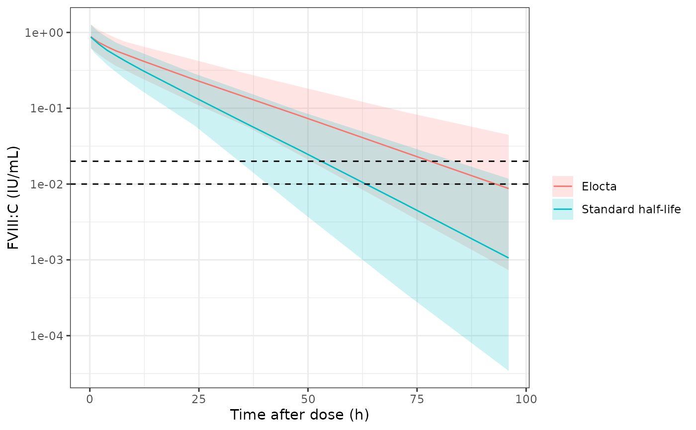
Simulated individual FVIII:C after 40 IU/kg on each product (median and 10th-90th percentile band); dashed lines mark 0.01 and 0.02 IU/mL troughs used in the paper’s clinical example.
Half-life after switching (Figure 6)
Figure 6 of the paper compares, for the 44 switchers, the half-life on the SHL product with the half-life on Elocta; the mean ratio was 1.48 and the multiple linear regression in Section 3.6 attributed +4.8 h to the switch, +0.13 h per year of age and -0.055 h per kg of weight.
hl_ind <- cohort |>
  mutate(
    cl = exp(ini_est[["lcl"]] + etalcl) * (WT / 64)^0.75 * (AGE / 30)^ini_est[["e_age_cl"]],
    vc = exp(ini_est[["lvc"]] + etalvc) * (WT / 64)^ini_est[["e_wt_vc"]],
    vp = exp(ini_est[["lvp"]] + etalvp),
    hl_shl = half_life_2cmt(cl, vc, q_typ, vp),
    hl_ehl = half_life_2cmt(cl * exp(ini_est[["e_form_fviii_fc_cl"]]), vc, q_typ, vp),
    ratio = hl_ehl / hl_shl
  )

hl_ind |>
  select(subject, `Standard half-life` = hl_shl, Elocta = hl_ehl) |>
  pivot_longer(-subject, names_to = "product", values_to = "hl") |>
  mutate(product = factor(product, c("Standard half-life", "Elocta"))) |>
  ggplot(aes(product, hl, group = subject)) +
  geom_line(alpha = 0.2) +
  geom_point(alpha = 0.4) +
  labs(x = NULL, y = "Terminal half-life (h)") +
  theme_bw()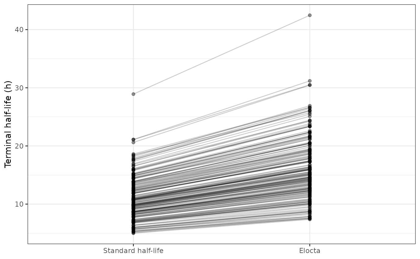
Replicates Figure 6 of Allard 2020: paired terminal half-lives of each virtual patient on a standard half-life product and on Elocta.
hl_ind |>
  summarise(
    `Median SHL t1/2 (h)` = median(hl_shl), `Median Elocta t1/2 (h)` = median(hl_ehl),
    `Mean ratio` = mean(ratio), `Median ratio` = median(ratio)
  ) |>
knitr::kable(digits = 2)| Median SHL t1/2 (h) | Median Elocta t1/2 (h) | Mean ratio | Median ratio |
|---|---|---|---|
| 10.45 | 15.12 | 1.46 | 1.47 |
reg_data <- bind_rows(
  hl_ind |> transmute(hl = hl_shl, switch = 0, AGE, WT),
  hl_ind |> transmute(hl = hl_ehl, switch = 1, AGE, WT)
)
fit <- lm(hl ~ switch + AGE + WT, data = reg_data)
knitr::kable(
  tibble(
    Term = c("Switch to Elocta (h)", "Age (h/year)", "Weight (h/kg)"),
    `Allard 2020 Section 3.6` = c(4.8, 0.13, -0.055),
    Simulated = unname(coef(fit)[c("switch", "AGE", "WT")])
  ),
  digits = 3
)| Term | Allard 2020 Section 3.6 | Simulated |
|---|---|---|
| Switch to Elocta (h) | 4.800 | 5.062 |
| Age (h/year) | 0.130 | 0.078 |
| Weight (h/kg) | -0.055 | 0.017 |
stopifnot(
  abs(median(hl_ind$ratio) - 1.48) < 0.05,
  coef(fit)[["switch"]] > 3, coef(fit)[["switch"]] < 7,
  coef(fit)[["AGE"]] > 0
)
With no within-patient (between-occasion) variability in the model, every virtual patient’s half-life is longer on Elocta; the four switchers (9%) whose observed half-life fell after switching reflect occasion-to-occasion variation and estimation noise in sparse routine data that the model does not describe. The regression on the simulated patients reproduces the switch effect and the direction of the age effect. The weight coefficient is not asserted: in the paper it came from the 44 switchers only, and in the model the weight exponents on CL (0.75) and V1 (0.827) nearly cancel in the half-life.
PKNCA validation
NCA on the noise-free individual profiles, grouped by product.
conc <- sim |>
  filter(!is.na(Cc)) |>
  select(id, time, Cc, product)
dose_df <- events |>
  filter(evid == 1L) |>
  select(id, time, amt, product)

conc_obj <- PKNCAconc(conc, Cc ~ time | product + id)
dose_obj <- PKNCAdose(dose_df, amt ~ time | product + id)
intervals <- data.frame(
  start = 0, end = Inf,
  cmax = TRUE, tmax = TRUE, aucinf.obs = TRUE, half.life = TRUE, cl.obs = TRUE
)
nca <- pk.nca(PKNCAdata(conc_obj, dose_obj, intervals = intervals))

nca_summary <- as.data.frame(nca$result) |>
  filter(PPTESTCD %in% c("cmax", "aucinf.obs", "half.life", "cl.obs")) |>
  group_by(product, PPTESTCD) |>
  summarise(median = median(PPORRES, na.rm = TRUE), .groups = "drop") |>
  pivot_wider(names_from = PPTESTCD, values_from = median)
nca_summary |>
  dplyr::rename(
    Product = product,
    "Cmax (IU/mL)" = cmax,
    "AUC0-inf (IU*h/mL)" = aucinf.obs,
    "t1/2 (h)" = half.life,
    "CL (mL/h)" = cl.obs
  ) |>
knitr::kable(digits = 3)| Product | AUC0-inf (IU*h/mL) | CL (mL/h) | Cmax (IU/mL) | t1/2 (h) |
|---|---|---|---|---|
| Elocta | 16.370 | 137.665 | 0.908 | 15.059 |
| Standard half-life | 11.042 | 204.089 | 0.908 | 10.402 |
The paper does not tabulate NCA results. The one comparable figure is the Discussion’s median Elocta half-life of 14.8 h among the study patients (the same model’s individual estimates), which the simulated cohort median is compared against below. The cohort is only an approximation of Table 1, so a difference of up to 20% is expected.
cmp <- ncaComparisonTable(
  simulated = as.data.frame(nca$result) |> filter(product == "Elocta"),
  reference = data.frame(half.life = 14.8),
  params = "half.life",
  units = c(half.life = "h")
)
knitr::kable(cmp)| NCA parameter | Reference | Simulated | % diff |
|---|---|---|---|
| t½ (h) | 14.8 | 15.1 | +1.7% |
Clinical example (Figure 7)
Section 5 illustrates dose individualisation for a 21-year-old, 105 kg man on Afstyla (a standard half-life product) dosed every 48 h. His individual parameters (Figure 7A) are empirical Bayes estimates that are not printed, so the typical-value profile for his covariates is shown instead of his own.
ev_ex <- lapply(c(1000, 2000), function(d) {
  rxode2::et(amt = d, ii = 48, addl = 9, cmt = "central") |>
    rxode2::et(seq(0, 480, by = 1), cmt = "central") |>
    as.data.frame() |>
    mutate(id = ifelse(d == 1000, 1L, 2L), regimen = paste(d, "IU q48h"))
}) |>
  bind_rows() |>
  mutate(WT = 105, AGE = 21, FORM_FVIII_FC = 0L)
sim_ex <- rxode2::rxSolve(rxode2::zeroRe(mod), ev_ex, keep = "regimen", returnType = "data.frame")
#> ℹ parameter labels from comments will be replaced by 'label()'
#> ℹ omega/sigma items treated as zero: 'etalcl', 'etalvc', 'etalvp'
#> Warning: multi-subject simulation without without 'omega'
sim_ex |>
  filter(time >= 384) |>
  ggplot(aes(time - 384, Cc, colour = regimen)) +
  geom_line() +
  geom_hline(yintercept = c(0.01, 0.02), linetype = "dashed") +
  scale_y_log10() +
  labs(x = "Time after dose at steady state (h)", y = "FVIII:C (IU/mL)", colour = NULL) +
  theme_bw()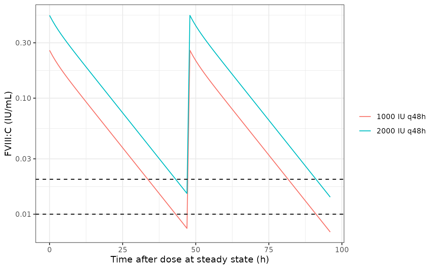
Typical-value FVIII:C for a 21-year-old, 105 kg patient on a standard half-life product at 1000 or 2000 IU every 48 h (compare Figure 7B-C of Allard 2020, which uses the patient’s individual estimates).
sim_ex |>
  filter(time == 480) |>
  select(regimen, `Trough FVIII:C (IU/mL)` = Cc) |>
knitr::kable(digits = 4)| regimen | Trough FVIII:C (IU/mL) |
|---|---|
| 1000 IU q48h | 0.007 |
| 2000 IU q48h | 0.014 |
The paper reports that this patient, with his individual estimates, stays above 0.01 IU/mL at 48 h on 1000 IU (1% risk of falling below) and above 0.02 IU/mL for 48 h on 2000 IU. The typical patient with his covariates has lower troughs than that, so his own clearance must be below the typical value. That is the paper’s argument for individual PK assessment, and the typical-value profile is not expected to reproduce it.
Assumptions and deviations
-
Signs of the age and Elocta coefficients. Table 2
prints both as negative (-0.214 and -0.394), with negative bootstrap
intervals, and the footnote equation
CLi = CLpop x (Age/30)^-0.214 x (weight/64)^0.75 x e^-0.394confirms it. Both directions agree with the reported longer half-life on Elocta and in older patients. -
Random-effect scale. Monolix reports omega as the
standard deviation of the random effect, so the Table 2 percentages are
read as omega = 0.349, 0.232 and 0.468 and squared to give the variances
in
ini(). The Corr(V1, Cl) row is a correlation coefficient, converted to a covariance. Q has no random effect (“fixed random effect” in the abstract). -
Residual error. Eq. 3 is the Monolix combined1
form, in which the additive and proportional standard deviations add
(
y = Cc + (a + b * Cc) * e), encoded withcombined1(). - Endogenous and residual FVIII. The authors fitted the data at steady state, adding four virtual prior doses at the known dosing interval to account for pre-dose (including endogenous) FVIII:C, and handled BLQ data as right-truncated. These are data-handling steps; the model has no endogenous production term (the authors tested one and did not retain it), so simulations start from zero FVIII:C.
-
Product indicator. The paper’s
EHLcovariate is encoded asFORM_FVIII_FC. Elocta was the only extended half-life product in the data, so the effect applies to the Fc-fusion product, not to other extended half-life FVIII concentrates. -
Screened covariates. von Willebrand factor, ABO
blood group and fat-free mass were tested but not retained (missing for
many patients); they are listed in
covariatesDataExcluded. Their estimates are in Supplementary Table S2, which is not used by the final model. - Virtual cohort. Age and weight distributions are approximations of Table 1; sex is not reported. No erratum was found in a Europe PMC search on 2026-09-26.