Praziquantel (Bustinduy 2016)
Source:vignettes/articles/Bustinduy_2016_praziquantel.Rmd
Bustinduy_2016_praziquantel.RmdModel and source
Citation: Bustinduy AL, Waterhouse D, de Sousa-Figueiredo JC, Roberts SA, Atuhaire A, Van Dam GJ, Corstjens PLAM, Scott JT, Stanton MC, Kabatereine NB, Ward S, Hope WW, Stothard JR. Population pharmacokinetics and pharmacodynamics of praziquantel in Ugandan children with intestinal schistosomiasis: higher dosages are required for maximal efficacy. mBio. 2016;7(4):e00227-16. doi:10.1128/mBio.00227-16. PMCID: PMC4992966.
Description: Two-compartment oral population PK model with a first-order absorption compartment and an absorption lag for TOTAL praziquantel (R-PZQ plus S-PZQ racemate) in 59 Ugandan children aged 3-8 years with egg-patent Schistosoma mansoni intestinal schistosomiasis, given a single oral dose of 40 or 60 mg/kg after a standardised breakfast. Fitted non-parametrically with the NPAG algorithm in Pmetrics 1.2.6. The authors describe the structure as three compartments (gut, central, peripheral); the gut is the absorption compartment, so in nlmixr2 terms this is a two-compartment disposition model with a depot. Clearance, central volume and the two intercompartmental rate constants Kcp (k12) and Kpc (k21) are primary parameters, each carrying its own inter-individual variability, as is the absorption lag. Oral bioavailability was NOT estimated, so clearance and volume are apparent (CL/F 608 L/h, V/F 474 L) and lfdepot is a fixed unit anchor. No covariate was retained: weight, age and sex were screened against the Bayesian posterior estimates and none showed a relationship, so the base model is the final model. Residual unexplained variability is carried as fixed(0) because the Pmetrics assay-error polynomial was never published. The authors also fitted a separate enantiomer-specific (R and S) structural model, but reported its parameters as ‘data not shown’, so only the total-PZQ model is extractable. The companion logistic exposure-response model for parasitological cure is NOT encoded here because its intercept is unreported; see the vignette Errata.
Article: https://doi.org/10.1128/mBio.00227-16 (open access; PMCID
PMC4992966)
Bustinduy and colleagues report the first praziquantel (PZQ) PK-PD study in young children. Sixty Ugandan children aged 3-8 years with egg-patent Schistosoma mansoni were randomised 1:1 to a single oral dose of 40 or 60 mg/kg. Two structural population PK models were built in Pmetrics 1.2.6 using the non-parametric NPAG algorithm: one for total PZQ (the sum of the R and S enantiomers) and a second, enantiomer-specific model whose parameters the authors report as “data not shown”. Only the total-PZQ model is therefore extractable, and it is the model the authors themselves carried forward into their Monte Carlo dose-finding simulations.
Population
59 children entered the population PK analysis (60 were enrolled; one was withdrawn 6 h into sampling with falciparum malaria). Baseline characteristics come from Table 1 of the paper: age 3-8 years (arm means 6.4 and 6.3 years), weight 15-34 kg (arm means 21.8 and 23.0 kg), 63.3% female, all resident in the villages of Bugoigo and Walukuba on the shore of Lake Albert, Uganda. Baseline S. mansoni intensity by Kato-Katz was heavy (>400 eggs per gram) in 23 children, medium in 17 and light in 19. Comorbidity was common: 37 of 59 were anaemic and 45 of 59 had a positive malaria rapid diagnostic test; no child tested positive for HIV.
Each child received breakfast before dosing because food increases PZQ bioavailability, and venous samples were drawn at 0, 1, 2, 4, 6, 12 and 24 h. R-PZQ and S-PZQ were quantified separately by LC-MS/MS over a 5-1500 ng/mL linear range; this model was fitted to their sum.
The same information is available programmatically via
readModelDb("Bustinduy_2016_praziquantel")()$population.
| Field | Value |
|---|---|
| species | human |
| n_subjects | 59 |
| n_studies | 1 |
| age_range | 3-8 years |
| age_median | Means by arm: 6.4 years (40 mg/kg) and 6.3 years (60 mg/kg); median not reported |
| weight_range | 15-34 kg |
| weight_median | Means by arm: 21.8 kg (40 mg/kg) and 23.0 kg (60 mg/kg); median not reported |
| sex_female_pct | 63.3 |
| race_ethnicity | Not reported (Ugandan children from Bugoigo and Walukuba villages on the shore of Lake Albert) |
| disease_state | Egg-patent Schistosoma mansoni intestinal schistosomiasis in a hyperendemic setting. Baseline intensity by Kato-Katz: heavy (>400 epg) 23 children, medium (100-399 epg) 17, light (1-100 epg) 19, and 1 child egg-negative but CCA-positive. Arithmetic mean baseline egg count 950.4 epg (40 mg/kg arm) and 491.0 epg (60 mg/kg arm). 37 of 59 were anaemic (haemoglobin < 11.5 g/dL) and 45 of 59 had a positive malaria rapid diagnostic test; no child tested positive for HIV. All children had received 40 mg/kg praziquantel at least one year before the study and had tolerated it. |
| dose_range | Single oral dose of praziquantel, randomised 1:1 to 40 mg/kg (n = 30) or 60 mg/kg (n = 30), administered after a breakfast of local foods because food increases PZQ bioavailability. |
| regions | Uganda (Bugoigo and Walukuba villages, Lake Albert) |
| notes | Baseline demographics from Bustinduy 2016 Table 1 (60 enrolled). 59 children completed the protocol and entered the population PK analysis (one child was withdrawn 6 h into sampling with falciparum malaria); 58 were available at the 24-day pharmacodynamic follow-up. Venous samples were drawn at 0, 1, 2, 4, 6, 12 and 24 h. R-PZQ and S-PZQ were quantified separately by LC-MS/MS, linear from 5 to 1500 ng/mL for each isomer; this model was fitted to their sum (total PZQ). Concentrations are in mg/L on the Fig. 3 observed-versus-predicted axes, while the Fig. 2 individual profiles and the Table 2 Cmax column are in ng/mL – the Table 2 header prints ‘ug/ml’ for Cmax, which is a unit typo; see the vignette Errata. |
Source trace
Every ini() entry carries an in-file comment naming its
source location; the table below collects them for review. All
structural values are the mean of the NPAG
non-parametric parameter distribution in Table 3.
| Equation / parameter | Value | Source location |
|---|---|---|
lka (Ka) |
14.89 1/h | Table 3, row K a (h-1), mean column (median 9.88) |
lcl (CL/F) |
608.02 L/h | Table 3, row SCL/F (liter/h), mean column (median
677.59) |
lvc (V/F) |
473.97 L | Table 3, row V/F (liter), mean column (median
503.90) |
lk12 (Kcp) |
25.90 1/h | Table 3, row K cp (h-1), mean column (median
22.28) |
lk21 (Kpc) |
33.30 1/h | Table 3, row K pc (h-1), mean column (median
25.71) |
ltlag (Tlag) |
1.94 h | Table 3, row T lag (h), mean column (median 1.67) |
lfdepot (F) |
fixed(log(1)) |
Methods: “Oral bioavailability was not estimated”; Table 3 footnote a |
etalka |
0.586965 | Table 3 CV% 89.36, as log(CV^2 + 1)
|
etalcl |
0.244672 | Table 3 CV% 52.65, as log(CV^2 + 1)
|
etalvc |
0.236472 | Table 3 CV% 51.65, as log(CV^2 + 1)
|
etalk12 |
0.426400 | Table 3 CV% 72.92, as log(CV^2 + 1)
|
etalk21 |
0.478345 | Table 3 CV% 78.32, as log(CV^2 + 1)
|
etaltlag |
0.292935 | Table 3 CV% 58.34, as log(CV^2 + 1)
|
propSd, addSd
|
fixed(0) |
Not reported anywhere in the paper; see Errata |
| ODE structure (gut / central / peripheral) | n/a | Methods, “Pharmacokinetic population analyses” |
alag(depot) |
n/a | Table 3 row T lag; Methods, “an absorption lag
(hours)” |
| No covariate retained | n/a | Results: “There was no relationship between any of the Bayesian estimates … Thus, the standard base model was used” |
Table 3 prints CV% alongside Mean and
SD, and SD / mean reproduces the printed
CV% for every row
(e.g. 320.10 / 608.02 = 52.65%), which confirms that the CV
is on the linear scale and fixes the
log(CV^2 + 1) conversion used above.
tab3 <- tibble::tribble(
  ~parameter, ~mean,   ~median, ~sd,    ~cv_pct,
  "Ka",        14.89,   9.88,   13.31,  89.36,
  "SCL/F",    608.02, 677.59,  320.10,  52.65,
  "V/F",      473.97, 503.90,  244.80,  51.65,
  "Kcp",       25.90,  22.28,   18.89,  72.92,
  "Kpc",       33.30,  25.71,   26.08,  78.32,
  "Tlag",       1.94,   1.67,    1.13,  58.34
) |>
  mutate(cv_from_sd_over_mean = 100 * sd / mean,
         omega2 = log((cv_pct / 100)^2 + 1))

# The printed CV% is SD/mean on the LINEAR scale, to within the 2-dp rounding of
# the printed SD. This is the fact that licences omega^2 = log(CV^2 + 1).
stopifnot(max(abs(tab3$cv_from_sd_over_mean - tab3$cv_pct)) < 0.15)

tab3 |>
  dplyr::rename(
    "Parameter"           = parameter,
    "Mean"                = mean,
    "Median"              = median,
    "SD"                  = sd,
    "CV% (printed)"       = cv_pct,
    "100 x SD/mean"       = cv_from_sd_over_mean,
    "omega^2 encoded"     = omega2
  ) |>
knitr::kable(digits = 4, caption = "Table 3 of Bustinduy 2016, with the CV% identity check.")| Parameter | Mean | Median | SD | CV% (printed) | 100 x SD/mean | omega^2 encoded |
|---|---|---|---|---|---|---|
| Ka | 14.89 | 9.88 | 13.31 | 89.36 | 89.3889 | 0.5870 |
| SCL/F | 608.02 | 677.59 | 320.10 | 52.65 | 52.6463 | 0.2447 |
| V/F | 473.97 | 503.90 | 244.80 | 51.65 | 51.6488 | 0.2365 |
| Kcp | 25.90 | 22.28 | 18.89 | 72.92 | 72.9344 | 0.4264 |
| Kpc | 33.30 | 25.71 | 26.08 | 78.32 | 78.3183 | 0.4783 |
| Tlag | 1.94 | 1.67 | 1.13 | 58.34 | 58.2474 | 0.2929 |
Structural verification
These checks are deterministic – they use typical values with the
random effects zeroed, so they do not depend on which cohort is drawn
and are gated tightly. They verify that the ODE system, the
q/vp routing, the absorption lag and the unit
bioavailability anchor are wired as the paper describes.
mod <- readModelDb("Bustinduy_2016_praziquantel")
mod_typ <- rxode2::zeroRe(mod)

# Analytic three-exponential solution for a two-compartment model with
# first-order absorption and an absorption lag, written directly from the
# micro-constants of Table 3. Independent of rxode2.
closed_form <- function(t, dose, ka, cl, vc, kcp, kpc, tlag) {
  k10   <- cl / vc
  s     <- k10 + kcp + kpc
  alpha <- (s + sqrt(s^2 - 4 * k10 * kpc)) / 2
  beta  <- (s - sqrt(s^2 - 4 * k10 * kpc)) / 2
  tp    <- pmax(t - tlag, 0)
  (dose * ka / vc) *
    ((kpc - ka)    / ((alpha - ka)    * (beta - ka))    * exp(-ka    * tp) +
     (kpc - alpha) / ((ka    - alpha) * (beta - alpha)) * exp(-alpha * tp) +
     (kpc - beta)  / ((ka    - beta)  * (alpha - beta)) * exp(-beta  * tp)) *
    (t >= tlag)
}

typ_profile <- function(dose) {
  ev <- rxode2::et(amt = dose, cmt = "depot") |>
    rxode2::et(seq(0, 24, by = 0.02), cmt = "central")
  # Tight tolerances: the closed form below is held to 1e-6, which the ODE
  # meets at rtol 1e-10 (3.8e-10) but not at the default 1e-6 (3.2e-5).
  rxode2::rxSolve(mod_typ, ev, returnType = "data.frame", rtol = 1e-10, atol = 1e-12)
}

dose40 <- 40 * 21.8   # arm mean weight, Table 1
dose60 <- 60 * 23.0
s40 <- typ_profile(dose40)
#> ℹ omega/sigma items treated as zero: 'etalka', 'etalcl', 'etalvc', 'etalk12', 'etalk21', 'etaltlag'
s60 <- typ_profile(dose60)
#> ℹ omega/sigma items treated as zero: 'etalka', 'etalcl', 'etalvc', 'etalk12', 'etalk21', 'etaltlag'

ref40 <- closed_form(s40$time, dose40, 14.89, 608.02, 473.97, 25.90, 33.30, 1.94)
ref60 <- closed_form(s60$time, dose60, 14.89, 608.02, 473.97, 25.90, 33.30, 1.94)
cf_err <- max(
  max(abs(s40$Cc - ref40)[ref40 > 1e-6] / ref40[ref40 > 1e-6]),
  max(abs(s60$Cc - ref60)[ref60 > 1e-6] / ref60[ref60 > 1e-6])
)

# The solved ODE must agree with the closed form to solver precision. This is
# what proves the peripheral compartment is actually in the system: routing the
# transfer through q = kcp * vc and vp = q / kpc rather than through the stored
# micro-constants keeps rxSolve()'s linCmt rewrite in agreement with the ODEs.
stopifnot(cf_err < 1e-6)

# The peripheral compartment is load-bearing: kill k12 and the profile moves.
# (An auto-solved one-compartment rewrite would leave it untouched.)
s_nok12 <- rxode2::rxSolve(mod_typ, rxode2::et(amt = dose40, cmt = "depot") |>
                             rxode2::et(seq(0, 24, by = 0.02), cmt = "central"),
                           returnType = "data.frame", rtol = 1e-10, atol = 1e-12,
                           params = c(lk12 = log(1e-9)))
#> ℹ omega/sigma items treated as zero: 'etalka', 'etalcl', 'etalvc', 'etalk12', 'etalk21', 'etaltlag'
k12_effect <- max(abs(s_nok12$Cc - s40$Cc) / pmax(s40$Cc, 1e-12))
stopifnot(k12_effect > 0.01)

# Absorption lag: nothing appears in plasma before Tlag.
stopifnot(all(s40$Cc[s40$time < 1.94] == 0))

# Mass balance with F anchored at 1: AUC(0-24) must recover Dose / CL, because
# the terminal half-life is ~1 h so 24 h is many half-lives.
auc40 <- PKNCA::pk.calc.auc.last(conc = s40$Cc, time = s40$time)
mb_err <- abs(auc40 / (dose40 / 608.02) - 1)
stopifnot(mb_err < 0.01)

# The model is linear, so exposure is exactly dose-proportional.
auc60 <- PKNCA::pk.calc.auc.last(conc = s60$Cc, time = s60$time)
prop_ratio <- (auc60 / dose60) / (auc40 / dose40)
stopifnot(abs(prop_ratio - 1) < 0.01)

tibble::tibble(
  Check = c("Solved ODE vs analytic three-exponential (max rel. error)",
            "Peripheral compartment is active (max rel. change when k12 -> 0)",
            "AUC(0-24) recovers Dose/CL (rel. error)",
            "Dose proportionality of AUC/dose, 60 vs 40 mg/kg"),
  Value = c(signif(cf_err, 3), signif(k12_effect, 3),
            signif(mb_err, 3), signif(prop_ratio, 6))
) |>
knitr::kable(caption = "Deterministic structural checks (all gated).")| Check | Value |
|---|---|
| Solved ODE vs analytic three-exponential (max rel. error) | 0.000000 |
| Peripheral compartment is active (max rel. change when k12 -> 0) | 1.000000 |
| AUC(0-24) recovers Dose/CL (rel. error) | 0.000642 |
| Dose proportionality of AUC/dose, 60 vs 40 mg/kg | 1.000000 |
The typical-value profiles peak at 0.884 mg/L (40 mg/kg) and 1.399 mg/L (60 mg/kg), both at 2.14 h. Those are population predictions, and they are the quantity plotted on the x-axis of the paper’s Figure 3A, whose range runs from 0 to about 1.5-2 mg/L. Reproducing that range is the positive check that Table 3 was transcribed correctly – see the Figure 3 section below.
Virtual cohort
Original subject-level data are not publicly available. The cohort below matches the weight distribution of Table 1: arm means of 21.8 and 23.0 kg over ranges of 15-30 and 15.1-34 kg. Weight enters only through the mg/kg dose, because the authors retained no covariate on any PK parameter.
# set.seed() seeds R's RNG. It does NOT seed rxode2's simulation RNG, and
# rxode2's streams are partitioned per solver thread, so the cohort below is
# reproducible on this machine and different on one with a different thread
# count. Every assertion downstream is written to hold for ANY cohort.
set.seed(20160809)

n_per_arm <- 200L   # the per-arm cohort cap; ample for this comparison

rtnorm <- function(n, mean, sd, lo, hi) {
  x <- stats::rnorm(n * 20, mean, sd)
  x <- x[x >= lo & x <= hi]
  stopifnot(length(x) >= n)
  x[seq_len(n)]
}

make_cohort <- function(n, mgkg, wt_mean, wt_lo, wt_hi, label, id_offset = 0L) {
  subj <- tibble::tibble(
    id        = id_offset + seq_len(n),
    WT        = rtnorm(n, wt_mean, (wt_hi - wt_lo) / 4, wt_lo, wt_hi),
    treatment = label
  )
  # Dense early grid so Tmax and the distribution phase are resolved; the study
  # itself sampled only at 0, 1, 2, 4, 6, 12 and 24 h.
  tgrid <- c(seq(0, 10, by = 0.05), seq(10.25, 24, by = 0.25))
  dplyr::bind_rows(
    subj |> dplyr::mutate(time = 0, amt = mgkg * WT, evid = 1L, cmt = "depot"),
    subj |> tidyr::crossing(time = tgrid) |>
      dplyr::mutate(amt = NA_real_, evid = 0L, cmt = "central")
  ) |>
    dplyr::arrange(id, time, dplyr::desc(evid))
}

events <- dplyr::bind_rows(
  make_cohort(n_per_arm, 40, 21.8, 15.0, 30.0, "40 mg/kg", id_offset = 0L),
  make_cohort(n_per_arm, 60, 23.0, 15.1, 34.0, "60 mg/kg", id_offset = n_per_arm)
)
stopifnot(!anyDuplicated(unique(events[, c("id", "time", "evid")])))
Simulation
sim <- rxode2::rxSolve(mod, events = events, keep = c("WT", "treatment")) |>
  as.data.frame()
# A numerically integrated ODE can undershoot zero by about its absolute
# tolerance (1e-8) on a decaying tail; NA would mean a subject failed to solve.
stopifnot(nrow(sim) > 0, !anyNA(sim$Cc), all(sim$Cc >= -1e-7))
Replicate published figures
# Corresponds to Figure 2 of Bustinduy 2016. The published panels show S-PZQ (A)
# and R-PZQ (B) SEPARATELY; this model is fitted to their SUM, so these curves
# should be compared against the sum of the two published panels. The paper's
# axes are ng/mL, so the simulated mg/L values are scaled by 1000. Thirty
# subjects per arm are shown, matching the published n per arm.
show_ids <- sim |>
  dplyr::distinct(id, treatment) |>
  dplyr::group_by(treatment) |>
  dplyr::slice_head(n = 30) |>
  dplyr::pull(id)

sim |>
  dplyr::filter(id %in% show_ids, !is.na(Cc)) |>
  ggplot(aes(time, 1000 * Cc, group = id, colour = treatment)) +
  geom_line(alpha = 0.6) +
  scale_colour_manual(values = c("40 mg/kg" = "#2166ac", "60 mg/kg" = "#b2182b")) +
  coord_cartesian(xlim = c(0, 24)) +
  labs(x = "Time (hours)", y = "Total PZQ concentration (ng/mL)",
       colour = NULL,
       caption = "Corresponds to Figure 2 of Bustinduy 2016 (published as S and R panels separately).")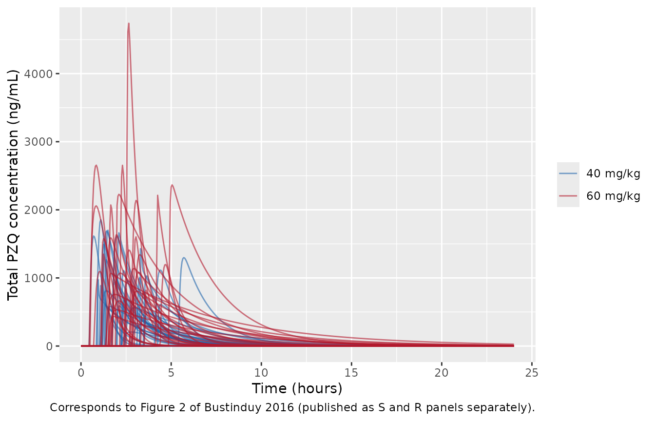
Individual total-PZQ profiles by dosing arm.
# Figure 3A of Bustinduy 2016 plots observed against POPULATION-predicted
# concentrations (i.e. before the Bayesian step), so its x-axis is generated with
# the Table 3 parameter vector and no between-subject variability. Its range runs
# from 0 to roughly 1.5-2 mg/L while the observed y-axis extends to 5 mg/L; that
# gap is the population-model bias the authors describe. Reproducing the x-axis
# range is the check that Table 3 was transcribed correctly.
pop_pred <- dplyr::bind_rows(
  dplyr::mutate(s40, treatment = "40 mg/kg"),
  dplyr::mutate(s60, treatment = "60 mg/kg")
)
pop_pred_max <- max(pop_pred$Cc)

# Figure 3A's x-axis spans 0 to 5 mg/L with every population prediction below
# about 2. A mis-transcribed CL, volume or dose unit moves this by a factor, not
# a few percent.
stopifnot(pop_pred_max > 0.5, pop_pred_max < 2.0)

ggplot(pop_pred, aes(time, Cc, colour = treatment)) +
  geom_line(linewidth = 0.9) +
  scale_colour_manual(values = c("40 mg/kg" = "#2166ac", "60 mg/kg" = "#b2182b")) +
  labs(x = "Time (hours)", y = "Population-predicted PZQ (mg/L)", colour = NULL,
       caption = "Population predictions from the Table 3 parameter vector; the x-axis quantity of Figure 3A.")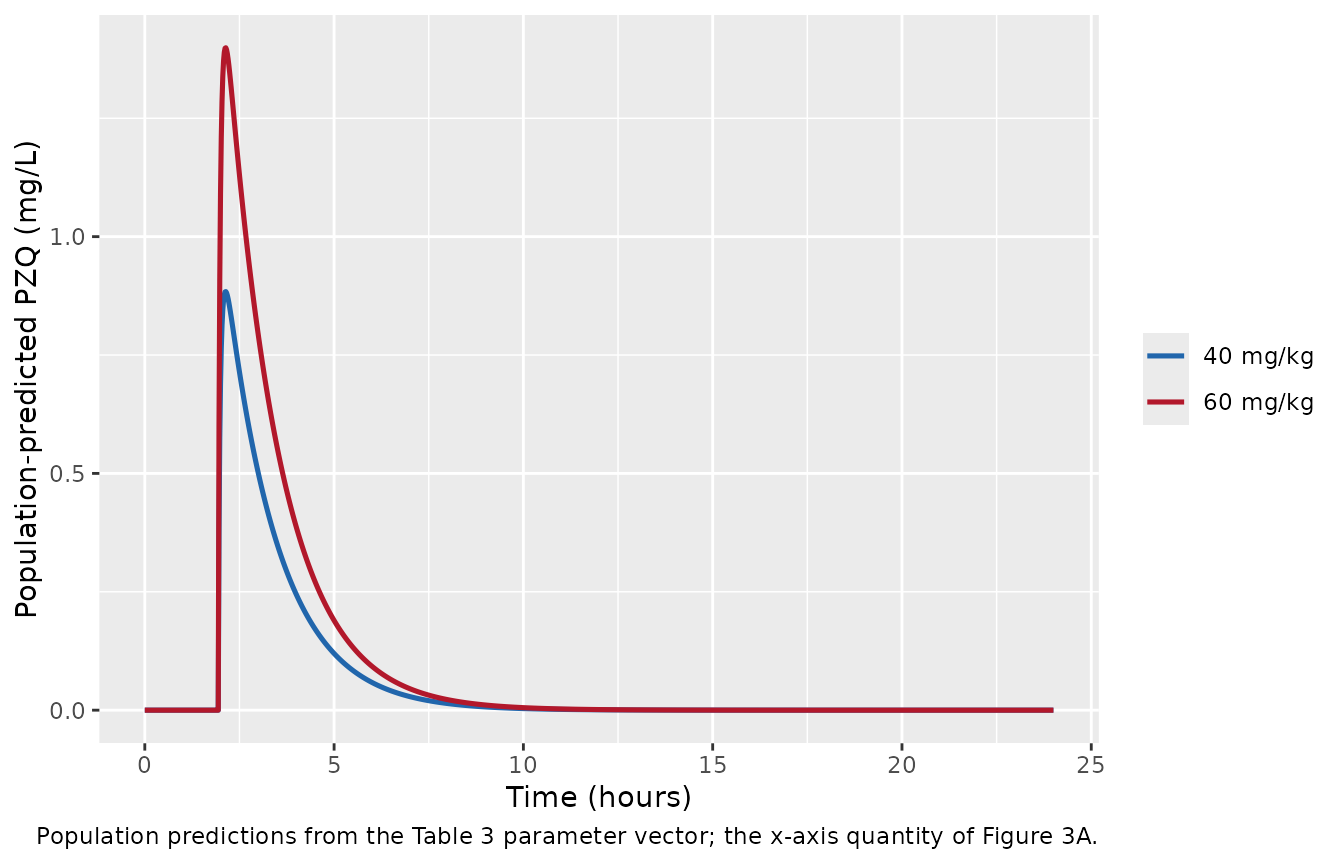
Population-predicted concentrations, the x-axis quantity of Figure 3A.
PKNCA validation
# Assay LLOQ: 5 ng/mL for each enantiomer, so 0.010 mg/L for their sum.
lloq <- 0.010

# Standard NCA BLQ handling: BLQ values BEFORE the peak are kept (they are true
# zeros during the absorption lag), BLQ values AFTER the peak are excluded. Note
# that dropping the pre-peak zeros instead would make PKNCA interpolate a
# straight line from (0, 0) to the first measurable point and inflate AUC by
# tens of percent -- the mass-balance gate below is what catches that.
sim_nca <- sim |>
  dplyr::filter(!is.na(Cc)) |>
  dplyr::group_by(id) |>
  dplyr::mutate(.tmax = time[which.max(Cc)]) |>
  dplyr::filter(time <= .tmax | Cc >= lloq) |>
  dplyr::ungroup() |>
  dplyr::select(id, time, Cc, treatment)

# Guarantee a time-zero row per subject; pre-dose Cc = 0 is correct for an
# extravascular dose.
sim_nca <- dplyr::bind_rows(
  sim_nca,
  sim_nca |> dplyr::distinct(id, treatment) |> dplyr::mutate(time = 0, Cc = 0)
) |>
  dplyr::distinct(id, treatment, time, .keep_all = TRUE) |>
  dplyr::arrange(id, treatment, time)

dose_df <- events |>
  dplyr::filter(evid == 1) |>
  dplyr::select(id, time, amt, treatment)

nca_res <- PKNCA::pk.nca(PKNCA::PKNCAdata(
  PKNCA::PKNCAconc(sim_nca, Cc ~ time | treatment + id),
  PKNCA::PKNCAdose(dose_df, amt ~ time | treatment + id),
  intervals = data.frame(start = 0, end = Inf, cmax = TRUE, tmax = TRUE,
                         aucinf.obs = TRUE, half.life = TRUE)
))

nca_long <- as.data.frame(nca_res)
stopifnot(nrow(nca_long) > 0, !all(is.na(nca_long$PPORRES)))
# Cohort mass balance: for this linear model AUC(0-inf) must equal Dose / CL for
# every subject. This is an identity, not a fit, so it is gated -- and it is the
# gate that goes red if the NCA input is ever filtered in a way that
# manufactures or destroys area.
mb <- nca_long |>
  dplyr::filter(PPTESTCD == "aucinf.obs") |>
  dplyr::select(id, auc = PPORRES) |>
  dplyr::left_join(
    sim |> dplyr::group_by(id) |> dplyr::summarise(cl = dplyr::first(cl), .groups = "drop"),
    by = "id"
  ) |>
  dplyr::left_join(dose_df |> dplyr::select(id, amt), by = "id") |>
  dplyr::mutate(ratio = auc / (amt / cl))

stopifnot(nrow(mb) == 2L * n_per_arm)
# Realised median 1.0002 with a 0.879-1.019 range over 400 subjects; the low tail
# is subjects whose peak sits close to the LLOQ so part of the curve is censored.
stopifnot(abs(stats::median(mb$ratio) - 1) < 0.01)
stopifnot(stats::quantile(abs(mb$ratio - 1), 0.9) < 0.05)
Comparison against published NCA
Table 2 of Bustinduy 2016 reports NCA parameters per enantiomer, as arithmetic means. This model describes their sum, so the reference row for each arm is built by adding the S and R entries. AUC adds exactly (the mean of a sum is the sum of the means); Cmax adds only approximately, but the two enantiomers share a Tmax to within 0.05 h so the approximation is close. Tmax cannot be summed and the S-PZQ value is used. There is no published total-PZQ half-life, so the S-PZQ value is carried as the closest available reference – S contributes 84% of the total AUC. The simulated side is summarised as the arithmetic mean so that it is compared like against like.
published <- tibble::tribble(
  ~treatment,  ~cmax,    ~tmax, ~aucinf.obs, ~half.life,
  # Cmax: Table 2 prints "ug/ml" but the values are ng/mL (see Errata); converted
  # to mg/L by dividing by 1000. 40 mg/kg: S 581.3 + R 131.1. 60: S 695.56 + R 144.95.
  "40 mg/kg",  0.71240,  3.33,  2.62 + 0.50, 2.96,
  "60 mg/kg",  0.84051,  3.23,  2.58 + 0.43, 3.02
)

simulated_mean <- nca_long |>
  dplyr::filter(PPTESTCD %in% c("cmax", "tmax", "aucinf.obs", "half.life")) |>
  dplyr::group_by(treatment, PPTESTCD) |>
  dplyr::summarise(value = mean(PPORRES, na.rm = TRUE), .groups = "drop") |>
  tidyr::pivot_wider(names_from = PPTESTCD, values_from = value)

cmp <- nlmixr2lib::ncaComparisonTable(
  simulated     = simulated_mean,
  reference     = published,
  by            = "treatment",
  units         = c(cmax = "mg/L", aucinf.obs = "mg*h/L", tmax = "h", half.life = "h"),
  tolerance_pct = 20
)

knitr::kable(
  cmp,
  digits  = 3,
  caption = paste(
    "Simulated (arithmetic mean over the virtual cohort) vs. Bustinduy 2016 Table 2",
    "totals. * differs from the reference by more than 20%. Every starred row is a",
    "known deviation discussed below, not a transcription error."
  )
)| NCA parameter | treatment | Reference | Simulated | % diff |
|---|---|---|---|---|
| Cmax (mg/L) | 40 mg/kg | 0.712 | 0.992 | +39.3%* |
| Cmax (mg/L) | 60 mg/kg | 0.841 | 1.45 | +73.1%* |
| Tmax (h) | 40 mg/kg | 3.33 | 2.53 | -24.0%* |
| Tmax (h) | 60 mg/kg | 3.23 | 2.47 | -23.5%* |
| AUC0-∞ (obs) (mg*h/L) | 40 mg/kg | 3.12 | 1.76 | -43.6%* |
| AUC0-∞ (obs) (mg*h/L) | 60 mg/kg | 3.01 | 2.78 | -7.6% |
| t½ (h) | 40 mg/kg | 2.96 | 1.56 | -47.3%* |
| t½ (h) | 60 mg/kg | 3.02 | 1.6 | -47.0%* |
Most rows are starred, and that is the expected result rather than a failure of the extraction. The authors say so themselves. Their Methods for the Monte Carlo simulation read:
Because of persistent bias when using the population parameter estimates (with both mean or median parameter values), we chose not to use these values and the associated population covariance matrix for the Monte Carlo simulations. Rather, we used the Bayesian posterior values for each patient.
Figure 3A shows that bias directly: population-predicted concentrations reach only about 1.5 mg/L while observations extend to 5 mg/L. A model built from the Table 3 parameter vector – which is the only parameter vector the paper publishes – inherits that bias exactly, and this vignette reproduces it rather than tuning it away. The individual Bayesian posteriors that the authors used instead are not published, so they cannot be packaged.
The direction of each deviation is informative:
- Half-life is about half the published value in both arms. The Table 3 micro-constants give a terminal rate constant of 0.715 1/h, i.e. a terminal half-life near 1 h, whereas the published NCA half-lives are 3.0-4.4 h. The study sampled at 0, 1, 2, 4, 6, 12 and 24 h, and by 12 h the observed concentrations are at or below the assay LLOQ (Figure 2), so the published terminal slopes rest on very few measurable points near the limit of quantification.
- AUC is under-predicted and Cmax over-predicted at the same time, which is the signature of a profile that is too peaked and decays too fast – the same short half-life seen from the other side.
- The 60 mg/kg arm deviates more than the 40 mg/kg arm. The published arm means are not dose-proportional at all (total AUC 3.12 at 40 mg/kg versus 3.01 at 60 mg/kg, i.e. slightly lower at the higher dose), whereas this model is strictly linear and therefore exactly proportional. That non-proportionality is the paper’s central finding – “dose is a notoriously inaccurate measure of actual drug exposure” – and with n = 30 per arm and a concentration CV above 100% the published arm means are themselves imprecise. A pooled-fit linear model cannot reproduce it and should not be made to.
These deviations are recorded, not gated: they are reproducible properties of the published parameter vector, so widening a tolerance until they disappear would only hide them.
Assumptions and deviations
-
Structural values are the Table 3 mean, not the
median. Table 3 prints both. The mean is used, matching the
sibling Pmetrics/NPAG extraction
Setiawan_2023_sulbactam. For CL and V the reported mean lies below the reported median (608.02 vs 677.59 L/h; 473.97 vs 503.90 L), so the underlying non-parametric distribution is left-skewed and no log-normal can reproduce both summaries at once. Substituting the medians does not improve the comparison above: it raises CL and lowers AUC further, and leaves the terminal rate constant essentially unchanged (0.712 vs 0.715 1/h). -
IIV is a log-normal approximation to a non-parametric
distribution. NPAG estimates a discrete set of support points,
not a parametric omega. The Table 3
CV%column is carried asomega^2 = log(CV^2 + 1). The CV% identity check above confirms the CV is on the linear scale. Off-diagonal covariances are not reported, so the etas are encoded as independent; in reality CL and V in a PK model of this kind are usually correlated, which means the simulated spread of AUC and Cmax is wider than the true posterior spread. -
Residual unexplained variability is
fixed(0). Neither the Pmetrics assay-error polynomial nor a lambda/gamma term appears in the paper, and the only supplemental item is Figure S1 (a side-effect frequency plot). The value was not invented.CcfromrxSolve()is therefore an individual prediction with no residual error added. -
Oral bioavailability was not estimated, so
lfdepotisfixed(log(1))and clearance and volume are apparent (CL/F, V/F) exactly as the paper reports them. The mass-balance checks above confirm the anchor. -
No covariate is in the model. Weight, age and sex
were screened against the Bayesian posterior estimates and none was
retained, so the base model is the final model; they are recorded in
covariatesDataExcluded. Weight still sets the mg/kg dose. The Discussion notes that allometric 0.75 scaling on clearance “may well be the most appropriate scaling function” but was not estimable over the narrow 15-34 kg range studied. - The virtual cohort’s weight distribution is an assumption. Table 1 gives an arm mean and a range but no SD or shape, so weights are drawn from a normal truncated to the published range with SD set to one quarter of that range. Because no PK parameter depends on weight, this choice affects only the dose and therefore scales exposure linearly.
- The enantiomer-specific model is not extractable. The Methods state that a separate structural model was developed for the R and S isoforms but report it as “data not shown”, so no parameter values exist to transcribe.
- The logistic cure model is not encoded. See Errata.
Errata and source-reporting gaps
-
Table 2 Cmax unit typo. The Cmax column header
reads
C max (ug/ml)but the values (581.3, 131.1, 695.56, 144.95) are ng/mL. Three independent facts fix this: the assay is “linear in the range from 5 to 1,500 ng/ml”; the Figure 2 concentration axis is labelled ng/mL and tops out near 4200; and the Figure 3 axes are mg/L with observations reaching 5. The AUC column in the same table is in ug*h/mL, which is self-consistent with a Cmax in ng/mL and a ~3 h half-life. The reference table in this vignette therefore divides the published Cmax by 1000. - Table 2 Tmax parenthetical. The footnote says the parentheses for Tmax show a range, but the study sampled only at 0, 1, 2, 4, 6, 12 and 24 h, so an observed Tmax range of “2.7-3.9” is impossible; the interval is almost certainly a 95% confidence interval on the mean. Nothing in the model depends on this.
-
Residual error is unreported (see above), carried
as
fixed(0). -
The logistic exposure-response model for parasitological
cure cannot be reconstructed. Table 5 publishes odds ratios for
the cure model – total PZQ AUC (log) adjusted OR 2.24 (95% CI 1.15-4.37)
and baseline S. mansoni intensity adjusted OR 0.99 (0.98-1.00)
– and the Monte Carlo section describes “a cure model based on a
logistic regression fit to the cure rate that included baseline egg
number and total AUC”. Two things block encoding it:
- The intercept is not reported anywhere. Without it the model yields no absolute probability of cure, only a relative exposure-response slope. It is not in the text, the tables, the figure panels (Figures 1-5 were inspected at native resolution) or the single supplemental figure.
- The scale of the egg-count coefficient is internally inconsistent as printed. Read literally as an odds ratio per single egg per gram, an OR of 0.99 implies that a child at the 40 mg/kg arm’s mean baseline burden of 950 epg carries a logit penalty near -9.5, which is irreconcilable with the observed 70-82% cure rates. A per-100-epg reading is arithmetically compatible, but the paper does not say so.