Vedolizumab (Waterhouse 2024)
Source:vignettes/articles/Waterhouse_2024_vedolizumab.Rmd
Waterhouse_2024_vedolizumab.Rmd
library(nlmixr2lib)
library(PKNCA)
#>
#> Attaching package: 'PKNCA'
#> The following object is masked from 'package:stats':
#>
#>     filter
library(rxode2)
#> rxode2 5.1.8 using 2 threads (see ?getRxThreads)
#>   no cache: create with `rxCreateCache()`
library(dplyr)
#>
#> Attaching package: 'dplyr'
#> The following objects are masked from 'package:stats':
#>
#>     filter, lag
#> The following objects are masked from 'package:base':
#>
#>     intersect, setdiff, setequal, union
library(tidyr)
library(ggplot2)
Model and source
#> ℹ parameter labels from comments will be replaced by 'label()'
#> Warning: some etas defaulted to non-mu referenced, possible parsing error: etaiov_cl_1, etaiov_cl_2, etaiov_cl_3, etaiov_cl_4, etaiov_cl_5, etaiov_cl_6, etaiov_cl_7
#> as a work-around try putting the mu-referenced expression on a simple line
Citation: Waterhouse T, Baron K, Eure W, Chen C, Dirks NL, Jansson J, Akbari M, Mehrotra S. Population pharmacokinetic modeling of vedolizumab for graft-versus-host disease prophylaxis in adults with allogeneic hematopoietic stem cell transplant. Pharmacol Res Perspect. 2024;12(5):e1257. doi:10.1002/prp2.1257.
Description: Two-compartment population PK model with first-order (linear) elimination for vedolizumab (humanised anti-alpha4-beta7 integrin IgG1 monoclonal antibody) as acute graft-versus-host disease (aGvHD) prophylaxis in adults undergoing allogeneic hematopoietic stem cell transplantation (allo-HSCT) (Waterhouse 2024).
Article: https://doi.org/10.1002/prp2.1257
Sibling model:
Rosario_2015_vedolizumab– the previous vedolizumab popPK developed in adults with ulcerative colitis and Crohn’s disease. Waterhouse 2024 refines that model for the allo-HSCT / GvHD prophylaxis setting, dropping the Michaelis-Menten pathway (unidentifiable in this dataset at 75-300 mg doses) and adding GvHD-organ / lymphocyte covariates.
Population
The model was developed on 193 evaluable adults undergoing allogeneic hematopoietic stem cell transplantation (allo-HSCT), pooled across two vedolizumab clinical studies: VEDO-1015 (phase 1b, NCT02728895, n=24, dose escalation from 75 to 300 mg IV) and VEDO-3035 GRAPHITE (phase 3, NCT03657160, n=169, 300 mg IV Q4W maintenance across seven scheduled dosing occasions). Baseline demographics (Waterhouse 2024 Table 1): age 18-72 years (mean 50.8, SD 14.9), body weight mean 78.5 kg (SD 19.1), 43.0% female, 74.1% White / 15.5% Asian / 2.1% Black / 8.3% not reported; mean baseline albumin 39.7 g/L (SD 5.60, i.e., ~3.97 g/dL) and mean baseline absolute lymphocyte count 426 cells/uL (SD 739). During the study, 3.1% of subjects developed liver aGvHD, 32.1% skin aGvHD, and 8.8% intestinal aGvHD (any grade, at any time). 76.7% of subjects received concomitant methotrexate, 56.0% tacrolimus, 44.0% cyclosporine, and 81.3% ursodeoxycholic acid.
The same information is available programmatically via
readModelDb("Waterhouse_2024_vedolizumab")()$population.
Source trace
The per-parameter origin is recorded as an in-file comment next to
each ini() entry in
inst/modeldb/specificDrugs/Waterhouse_2024_vedolizumab.R.
The table below collects them in one place.
| Equation / parameter | Value | Source location (Waterhouse 2024) |
|---|---|---|
lcl |
log(0.148) |
Table 2: CL = 0.148 L/day (95% CI 0.136-0.162, RSE 4.49%) |
lvc |
log(3.12) |
Table 2: Vc = 3.12 L (95% CI 3.03-3.21, RSE 1.44%) |
lq |
log(0.500) |
Table 2: Q = 0.500 L/day (95% CI 0.408-0.612, RSE 10.4%) |
lvp |
log(3.95) |
Table 2: Vp = 3.95 L (95% CI 3.52-4.44, RSE 5.93%) |
e_wt_cl |
0.713 |
Table 2: body weight effect on CL (95% CI 0.523-0.902) |
e_alb_cl |
-1.35 |
Table 2: albumin effect on CL (95% CI -1.67 to -1.02) |
e_lymph_cl |
-0.0180 |
Table 2: lymphocyte count effect on CL (95% CI -0.0524 to 0.0164) |
e_age_cl |
-0.130 |
Table 2: age effect on CL (95% CI -0.242 to -0.0185) |
e_wt_vc |
0.659 |
Table 2: body weight effect on Vc (95% CI 0.540-0.778) |
e_wt_vp |
fixed(1.00) |
Table 2 + Supp Eq S2: body weight effect on Vp = 1 Fixed |
e_wt_q |
fixed(0.75) |
Section 3.2.2 text + Supp Eq S2:
theta_11 for Q (fixed to 0.75). Table 2 prints
0.50 Fixed which contradicts the text and the supplement
equation and is treated as a typographical error (see Errata). |
e_liver_gvhd_cl |
1.05 |
Table 2: liver GvHD effect on CL (95% CI 0.834-1.26) |
e_skin_gvhd_cl |
1.03 |
Table 2: skin GvHD effect on CL (95% CI 0.940-1.12) |
e_intestine_gvhd_cl |
1.07 |
Table 2: intestine GvHD effect on CL (95% CI 0.870-1.27) |
IIV omega^2_CL
|
0.0827 |
Table 3: CV% = 29.4, 95% CI 0.0588-0.107 |
IIV omega^2_Vc
|
0.0323 |
Table 3: CV% = 18.1, 95% CI 0.0235-0.0411 |
IIV omega^2_Vp
|
0.179 |
Table 3: CV% = 44.2, 95% CI 0.0920-0.265 |
cov(CL, Vc) |
0.0214 |
Table 3: Corr = 0.415 |
cov(CL, Vp) |
-0.0253 |
Table 3: Corr = -0.208 |
cov(Vc, Vp) |
0.0272 |
Table 3: Corr = 0.358 |
propSd |
sqrt(0.0241) ~ 0.1553 |
Table 3: sigma^2_prop = 0.0241 (CV% = 15.5) |
IOV on CL etaiov_cl_1..7
|
omega^2 = 0.0315 |
Table 3: IOV-CL CV% = 17.9, 95% CI 0.0190-0.0440, shrinkage 55.4%. Occasion definition: Methods Section 2.2.2 |
| Model structure | 2-cmt linear elimination | Section 3.2.1 base model + Section 3.2.2 final model |
Reference patient (Waterhouse 2024 Table 2 and Table 3 footnote): 53-year-old subject weighing 75 kg with no aGvHD in liver, skin, or intestine, an albumin value of 40 g/L (equivalently 4 g/dL), and a lymphocyte count of 100 cells/uL (equivalently 0.1 K/uL).
Virtual cohort
Original observed data are not publicly available. The simulations below use a virtual population whose covariate distributions approximate the published demographics (Waterhouse 2024 Table 1). Cohort size is capped at 200 per arm.
make_cohort <- function(n,
                        n_doses               = 7,
                        first_dose_day        = 0,
                        second_dose_offset    = 14,
                        maintenance_interval  = 28,
                        obs_days_per_dose     = c(0, 0.02, 0.1, 1, 3, 7, 14, 21, 28),
                        amt_mg                = 300,
                        id_offset             = 0L,
                        seed                  = 12571) {
  set.seed(seed)

  # Baseline covariates approximating Waterhouse 2024 Table 1.
  WT              <- pmax(35, pmin(160, rlnorm(n, log(78.5), 0.24)))
  AGE             <- pmax(18, pmin(72,  rnorm(n, 50.8, 14.9)))
  ALB             <- pmax(20, pmin(60,  rnorm(n, 39.7, 5.60)))       # g/L (SI)
  # Absolute lymphocyte count in cells/uL (paper reports K/uL; multiply by 1000).
  LYMPH_ABS       <- pmax(0, exp(rnorm(n, log(200), 1.2)))
  AGVHD_LIVER     <- rbinom(n, 1, 0.031)
  AGVHD_SKIN      <- rbinom(n, 1, 0.321)
  AGVHD_INTESTINE <- rbinom(n, 1, 0.088)

  # Waterhouse 2024 phase 3 dose schedule: Days -1, +13, +41, +69, +97, +125, +153
  # relative to transplantation, which is:
  #   day 0        (first dose)
  #   day 14       (second dose, 14 days after the first)
  #   day 42, 70, 98, 126, 154 (Q4W maintenance thereafter)
  dose_times <- c(
    first_dose_day,
    first_dose_day + second_dose_offset,
    first_dose_day + second_dose_offset +
      maintenance_interval * seq_len(pmax(0, n_doses - 2))
  )

  pop <- data.frame(
    ID = id_offset + seq_len(n),
    WT, AGE, ALB, LYMPH_ABS,
    AGVHD_LIVER, AGVHD_SKIN, AGVHD_INTESTINE
  )

  infusion_days <- 0.5 / 24  # 30-minute IV infusion in days
  d_dose <- pop[rep(seq_len(n), each = length(dose_times)), ] |>
    mutate(
      TIME = rep(dose_times, times = n),
      AMT  = amt_mg,
      EVID = 1,
      CMT  = "central",
      RATE = amt_mg / infusion_days,
      DV   = NA_real_
    )

  obs_grid <- as.vector(outer(obs_days_per_dose, dose_times, "+"))
  obs_grid <- sort(unique(pmax(0, obs_grid)))

  d_obs <- pop[rep(seq_len(n), each = length(obs_grid)), ] |>
    mutate(
      TIME = rep(obs_grid, times = n),
      AMT  = 0,
      EVID = 0,
      CMT  = "central",
      RATE = 0,
      DV   = NA_real_
    )

  bind_rows(d_dose, d_obs) |>
    arrange(ID, TIME, desc(EVID)) |>
    # OCC: the dosing occasion each record belongs to (Waterhouse 2024 Methods
    # 2.2.2 -- a new occasion begins at each administered dose and runs until the
    # next dose). Records at or before the first dose take occasion 1.
    mutate(OCC = pmax(1L, findInterval(TIME, dose_times))) |>
    select(ID, TIME, AMT, EVID, CMT, RATE, DV, OCC,
           WT, AGE, ALB, LYMPH_ABS,
           AGVHD_LIVER, AGVHD_SKIN, AGVHD_INTESTINE)
}
mod <- rxode2::rxode(readModelDb("Waterhouse_2024_vedolizumab"))
#> ℹ parameter labels from comments will be replaced by 'label()'
#> Warning: some etas defaulted to non-mu referenced, possible parsing error: etaiov_cl_1, etaiov_cl_2, etaiov_cl_3, etaiov_cl_4, etaiov_cl_5, etaiov_cl_6, etaiov_cl_7
#> as a work-around try putting the mu-referenced expression on a simple line
Simulation
Phase 3 dosing (VEDO-3035 GRAPHITE): 300 mg IV Q4W for 7 doses (first two doses 14 days apart, then Q4W).
events_vpc <- make_cohort(n = 200)
sim_vpc <- rxode2::rxSolve(mod, events = events_vpc) |> as.data.frame()
Concentration-time VPC over the phase 3 dosing schedule
d_vpc <- sim_vpc |>
  group_by(time) |>
  summarise(
    Q05 = quantile(Cc, 0.05, na.rm = TRUE),
    Q50 = quantile(Cc, 0.50, na.rm = TRUE),
    Q95 = quantile(Cc, 0.95, na.rm = TRUE),
    .groups = "drop"
  )

ggplot(d_vpc, aes(x = time, y = Q50)) +
  geom_ribbon(aes(ymin = Q05, ymax = Q95), fill = "#4682b4", alpha = 0.25) +
  geom_line(colour = "#4682b4", linewidth = 0.8) +
  geom_line(aes(y = Q05), linetype = "dashed", linewidth = 0.4) +
  geom_line(aes(y = Q95), linetype = "dashed", linewidth = 0.4) +
  scale_y_log10() +
  labs(
    x = "Time since first dose (days)",
    y = "Vedolizumab concentration (ug/mL, log scale)",
    title = "Simulated concentration-time VPC over the phase 3 schedule",
    caption = paste0(
      "Simulated 5th / 50th / 95th percentiles, N = 200 virtual subjects, ",
      "300 mg IV over 30 min at days 0, 14, 42, 70, 98, 126, 154.\n",
      "Compare with Figure 4 (final model VPC) of Waterhouse 2024."
    )
  ) +
  theme_bw()
#> Warning in scale_y_log10(): log-10 transformation introduced infinite values.
#> log-10 transformation introduced infinite values.
#> log-10 transformation introduced infinite values.
#> log-10 transformation introduced infinite values.
#> log-10 transformation introduced infinite values.
#> log-10 transformation introduced infinite values.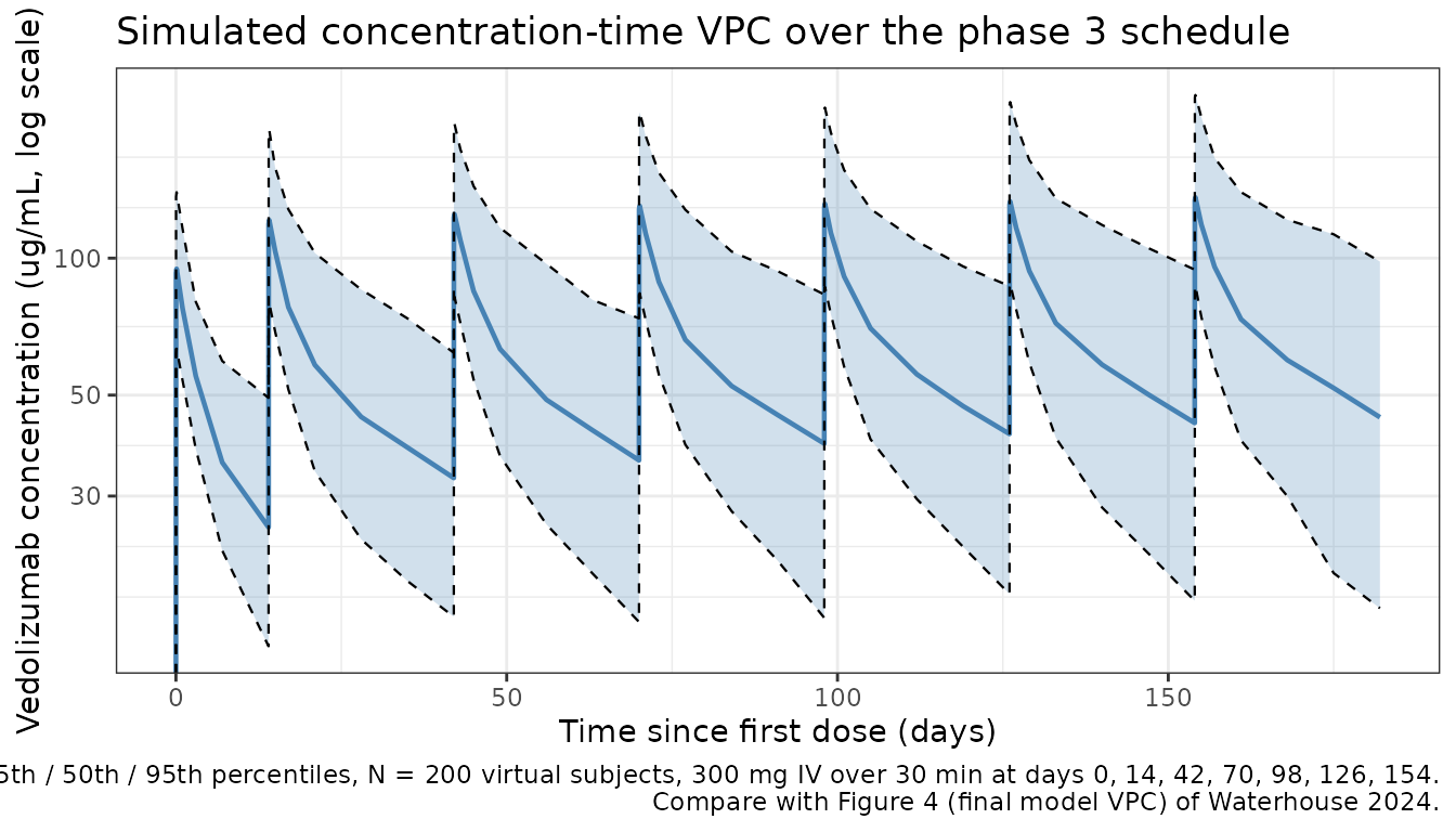
Inter-occasion variability on CL
Waterhouse 2024 estimates inter-occasion variability on CL (Table 3,
variance 0.0315, CV% 17.9). An occasion begins at each administered dose
and runs until the next (Methods Section 2.2.2), so the model requires
an OCC column in the event table;
make_cohort() above derives it from the dose schedule.
The check below is deterministic: all etas are supplied as event-data
columns with omega = NA, and only the occasion-2 IOV eta is
perturbed. Clearance must change during occasion 2 alone, leaving
occasion 1 untouched.
ev_iov <- make_cohort(n = 1, n_doses = 3) |>
  mutate(
    WT = 75, AGE = 53, ALB = 40, LYMPH_ABS = 100,
    AGVHD_LIVER = 0, AGVHD_SKIN = 0, AGVHD_INTESTINE = 0,
    etalcl = 0, etalvc = 0, etalvp = 0,
    etaiov_cl_1 = 0, etaiov_cl_2 = 0, etaiov_cl_3 = 0, etaiov_cl_4 = 0,
    etaiov_cl_5 = 0, etaiov_cl_6 = 0, etaiov_cl_7 = 0
  )

cl_by_occ <- function(events) {
  out <- rxode2::rxSolve(mod, events = events, omega = NA) |>
    as.data.frame()
  # CL is piecewise-constant within an occasion here (covariates and etas are
  # fixed), so the within-occasion spread must be numerically zero.
  stopifnot(max(tapply(out$cl, out$OCC, function(x) diff(range(x)))) < 1e-9)
  out |>
    group_by(OCC) |>
    summarise(CL = mean(cl), .groups = "drop")
}

cl_ref  <- cl_by_occ(ev_iov)
cl_pert <- cl_by_occ(ev_iov |> mutate(etaiov_cl_2 = log(2)))

iov_tbl <- left_join(cl_ref, cl_pert, by = "OCC", suffix = c("_ref", "_pert")) |>
  mutate(Ratio = CL_pert / CL_ref)

# Occasion 2 CL must double; all other occasions must be untouched.
stopifnot(
  isTRUE(all.equal(iov_tbl$Ratio[iov_tbl$OCC == 2], 2, tolerance = 1e-6)),
  isTRUE(all.equal(iov_tbl$Ratio[iov_tbl$OCC != 2],
                   rep(1, sum(iov_tbl$OCC != 2)), tolerance = 1e-6))
)

iov_tbl |>
  dplyr::rename(
    "Occasion"           = OCC,
    "CL, reference (L/day)" = CL_ref,
    "CL, eta_IOV,2 = log(2) (L/day)" = CL_pert,
    "Ratio"              = Ratio
  ) |>
  knitr::kable(
    caption = paste0(
      "IOV multiplexing check: perturbing the occasion-2 IOV eta changes CL ",
      "during occasion 2 only."
    )
)| Occasion | CL, reference (L/day) | CL, eta_IOV,2 = log(2) (L/day) | Ratio |
|---|---|---|---|
| 1 | 0.148 | 0.148 | 1 |
| 2 | 0.148 | 0.296 | 2 |
| 3 | 0.148 | 0.148 | 1 |
Covariate forest plot (final-model covariate effects on CL)
Waterhouse 2024 Figure 3 renders a covariate forest plot showing the multiplicative effect on clearance when each covariate moves from the reference value to the 5th/10th/25th/75th/90th/95th percentiles (continuous) or from 0 to 1 (categorical GvHD). We reproduce the equivalent multiplicative ratios from the model’s coefficients.
ini <- mod$theta
get <- function(nm) unname(ini[nm])

# Continuous covariate sensitivity at 5th / 95th population percentiles from
# the virtual cohort above (rough approximations of Waterhouse 2024 Figure 3
# reference-cohort percentiles).
forest_cont <- tribble(
  ~covariate,               ~low,   ~ref,   ~high,  ~exponent,
  "Weight (kg)",            51,     75,     105,    get("e_wt_cl"),
  "Albumin (g/L)",          31,     40,     46,     get("e_alb_cl"),
  "Lymphocyte (cells/uL)",  10,     100,    2000,   get("e_lymph_cl"),
  "Age (years)",            23,     53,     67,     get("e_age_cl")
) |>
  mutate(
    ratio_low  = (low  / ref)^exponent,
    ratio_high = (high / ref)^exponent
  )

forest_cat <- tribble(
  ~covariate,                    ~ratio_low, ~ratio_high,
  "Liver aGvHD (vs none)",       1,           get("e_liver_gvhd_cl"),
  "Skin aGvHD (vs none)",        1,           get("e_skin_gvhd_cl"),
  "Intestinal aGvHD (vs none)",  1,           get("e_intestine_gvhd_cl")
)

forest_all <- bind_rows(
  forest_cont |> select(covariate, ratio_low, ratio_high),
  forest_cat
) |>
  mutate(covariate = factor(covariate, levels = rev(covariate)))

ggplot(forest_all, aes(y = covariate)) +
  geom_segment(aes(x = ratio_low, xend = ratio_high, yend = covariate),
               colour = "#4682b4", linewidth = 1.0) +
  geom_point(aes(x = ratio_low),  colour = "#4682b4", size = 2) +
  geom_point(aes(x = ratio_high), colour = "#4682b4", size = 2) +
  geom_vline(xintercept = 1, linetype = "dashed", colour = "grey40") +
  geom_vline(xintercept = c(0.75, 1.25), linetype = "dotted", colour = "grey60") +
  scale_x_log10(breaks = c(0.5, 0.75, 1.0, 1.25, 1.5, 2.0)) +
  labs(
    x = "Multiplicative effect on CL relative to reference",
    y = NULL,
    title = "Covariate effects on vedolizumab CL",
    caption = paste0(
      "Ratios computed at the 5th / 95th covariate percentiles vs the reference.\n",
      "Reference (Waterhouse 2024 Table 2): 75 kg, 53 y, albumin 40 g/L, ",
      "lymphocyte 100 cells/uL, no aGvHD."
    )
  ) +
  theme_bw()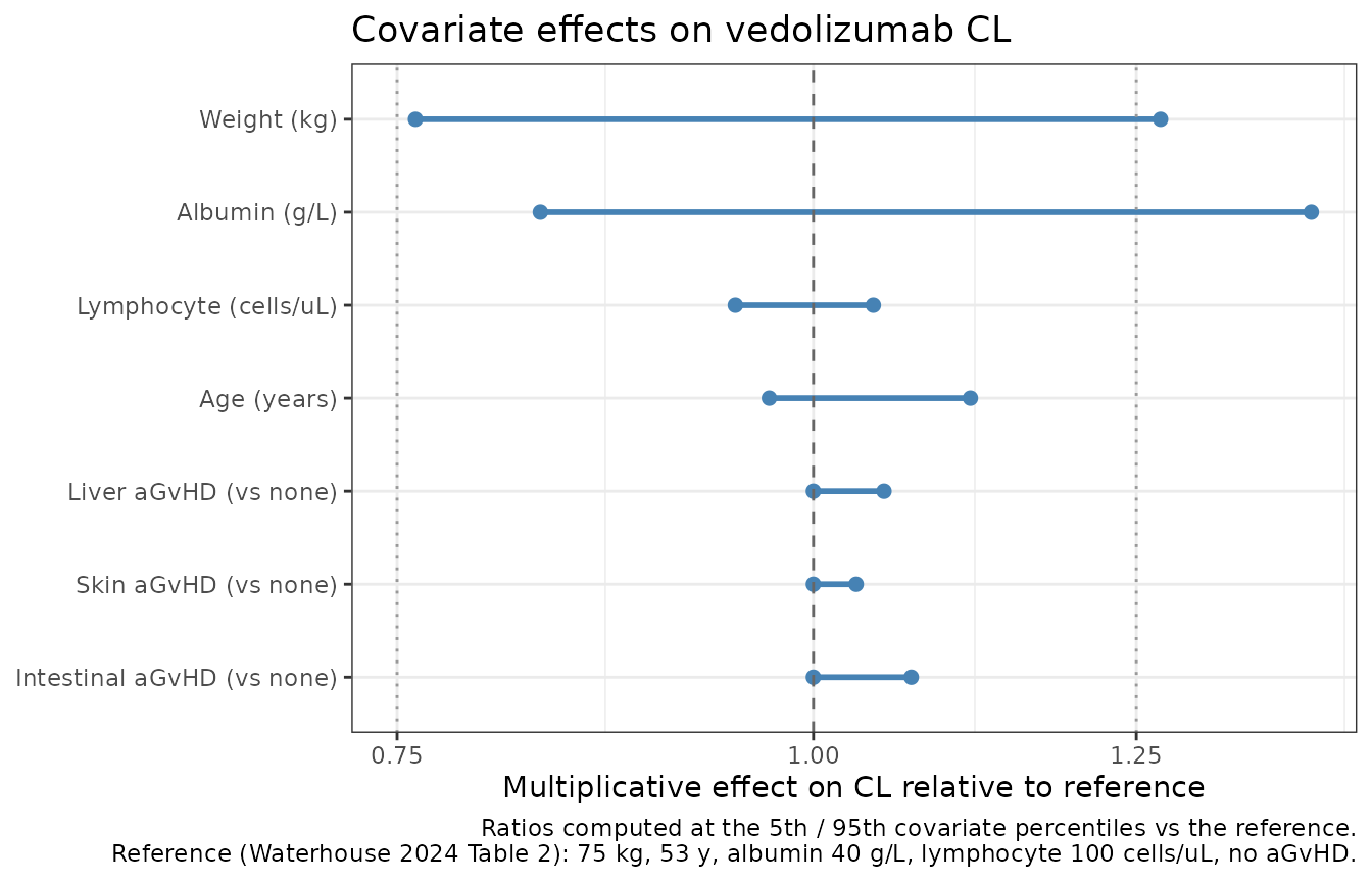
The paper’s clinical-meaningfulness band is +/-25% (dotted lines). Only albumin and body-weight excursions cross this band – consistent with the paper’s conclusion that these are the only clinically important predictors of vedolizumab CL in this population.
PKNCA validation
We compute NCA on a typical-patient profile (reference covariates)
after a single 300 mg IV dose and at steady state (dose 7 of the phase 3
regimen). The paper reports no explicit reference-patient NCA table, so
this section serves primarily as a sanity check: derived Cmax after a
30-minute infusion should be close to
dose / Vc ~ 300 mg / 3.12 L ~ 96 ug/mL and the terminal
half-life should be in the range typical of therapeutic IgG1 mAbs
(roughly 20-35 days).
mod_typical <- mod |> rxode2::zeroRe()
#> Warning: some etas defaulted to non-mu referenced, possible parsing error: etaiov_cl_1, etaiov_cl_2, etaiov_cl_3, etaiov_cl_4, etaiov_cl_5, etaiov_cl_6, etaiov_cl_7
#> as a work-around try putting the mu-referenced expression on a simple line

events_single <- make_cohort(
  n = 1,
  n_doses = 1,
  obs_days_per_dose = c(0, 0.02, 0.1, 0.25, 0.5, 1, 2, 4, 7, 14, 21, 28,
                        42, 56, 84, 112, 168, 224)
) |>
  mutate(
    WT = 75, AGE = 53, ALB = 40, LYMPH_ABS = 100,
    AGVHD_LIVER = 0, AGVHD_SKIN = 0, AGVHD_INTESTINE = 0
  )

sim_single <- rxode2::rxSolve(mod_typical, events = events_single) |>
  as.data.frame() |>
  mutate(id = 1L, treatment = "single_300mg")
#> ℹ omega/sigma items treated as zero: 'etalcl', 'etalvc', 'etalvp', 'etaiov_cl_1', 'etaiov_cl_2', 'etaiov_cl_3', 'etaiov_cl_4', 'etaiov_cl_5', 'etaiov_cl_6', 'etaiov_cl_7'

sim_nca_single <- sim_single |>
  filter(!is.na(Cc)) |>
  select(id, time, Cc, treatment)

sim_nca_single <- bind_rows(
  sim_nca_single,
  sim_nca_single |> distinct(id, treatment) |>
    mutate(time = 0, Cc = 0)
) |>
  distinct(id, treatment, time, .keep_all = TRUE) |>
  arrange(id, treatment, time)

dose_single <- events_single |>
  filter(EVID == 1) |>
  transmute(id = ID, time = TIME, amt = AMT, treatment = "single_300mg")

conc_single <- PKNCA::PKNCAconc(sim_nca_single, Cc ~ time | treatment + id)
dose_single_obj <- PKNCA::PKNCAdose(dose_single, amt ~ time | treatment + id)

intervals_single <- data.frame(
  start      = 0,
  end        = Inf,
  cmax       = TRUE,
  tmax       = TRUE,
  aucinf.obs = TRUE,
  half.life  = TRUE
)

nca_single <- PKNCA::pk.nca(
  PKNCA::PKNCAdata(conc_single, dose_single_obj, intervals = intervals_single)
)
as.data.frame(nca_single$result) |>
  dplyr::rename(
    "Group"     = treatment,
    "Subject"   = id,
    "PPTESTCD"  = PPTESTCD,
    "Value"     = PPORRES
  ) |>
  knitr::kable(
    caption = "Single-dose NCA on the typical reference-patient profile."
)| Group | Subject | start | end | PPTESTCD | Value | exclude |
|---|---|---|---|---|---|---|
| single_300mg | 1 | 0 | Inf | cmax | 121.8039095 | NA |
| single_300mg | 1 | 0 | Inf | tmax | 14.1000000 | NA |
| single_300mg | 1 | 0 | Inf | tlast | 238.0000000 | NA |
| single_300mg | 1 | 0 | Inf | clast.obs | 0.8648742 | NA |
| single_300mg | 1 | 0 | Inf | lambda.z | 0.0190734 | NA |
| single_300mg | 1 | 0 | Inf | r.squared | 0.9999913 | NA |
| single_300mg | 1 | 0 | Inf | adj.r.squared | 0.9999905 | NA |
| single_300mg | 1 | 0 | Inf | lambda.z.time.first | 28.0000000 | NA |
| single_300mg | 1 | 0 | Inf | lambda.z.time.last | 238.0000000 | NA |
| single_300mg | 1 | 0 | Inf | lambda.z.n.points | 13.0000000 | NA |
| single_300mg | 1 | 0 | Inf | clast.pred | 0.8633641 | NA |
| single_300mg | 1 | 0 | Inf | half.life | 36.3410273 | NA |
| single_300mg | 1 | 0 | Inf | span.ratio | 5.7785928 | NA |
| single_300mg | 1 | 0 | Inf | aucinf.obs | 4071.8651409 | NA |
# Phase 3 dosing: seven doses at days 0, 14, 42, 70, 98, 126, 154.
# Steady state is well approached by dose 7 (day 154). Extract the final
# dosing interval (day 154 to day 182) plus the extrapolation window used
# for AUC-inf and half-life.
final_dose_day <- 154

events_ss_base <- make_cohort(
  n = 1, n_doses = 7,
  obs_days_per_dose = c(0, 0.02, 0.1, 0.5, 1, 2, 4, 7, 14, 21, 28),
  first_dose_day = 0
) |>
  mutate(
    WT = 75, AGE = 53, ALB = 40, LYMPH_ABS = 100,
    AGVHD_LIVER = 0, AGVHD_SKIN = 0, AGVHD_INTESTINE = 0
  )

extra_obs <- data.frame(
  ID = 1L,
  TIME = final_dose_day + c(35, 42, 56, 84, 112, 168, 224),
  AMT = 0, EVID = 0, CMT = "central", RATE = 0, DV = NA_real_,
  OCC = 7L,  # washout observations belong to the seventh (final) dosing occasion
  WT = 75, AGE = 53, ALB = 40, LYMPH_ABS = 100,
  AGVHD_LIVER = 0, AGVHD_SKIN = 0, AGVHD_INTESTINE = 0
)
events_ss <- bind_rows(events_ss_base, extra_obs) |>
  arrange(ID, TIME, desc(EVID))

sim_ss <- rxode2::rxSolve(mod_typical, events = events_ss) |>
  as.data.frame() |>
  mutate(id = 1L, treatment = "ss_300mg_final_dose")
#> ℹ omega/sigma items treated as zero: 'etalcl', 'etalvc', 'etalvp', 'etaiov_cl_1', 'etaiov_cl_2', 'etaiov_cl_3', 'etaiov_cl_4', 'etaiov_cl_5', 'etaiov_cl_6', 'etaiov_cl_7'

sim_nca_ss <- sim_ss |>
  filter(!is.na(Cc), time >= final_dose_day) |>
  mutate(time = time - final_dose_day) |>
  select(id, time, Cc, treatment)

sim_nca_ss <- bind_rows(
  sim_nca_ss,
  sim_nca_ss |> distinct(id, treatment) |>
    mutate(time = 0, Cc = min(sim_nca_ss$Cc[sim_nca_ss$time == 0], na.rm = TRUE))
) |>
  distinct(id, treatment, time, .keep_all = TRUE) |>
  arrange(id, treatment, time)

dose_ss <- data.frame(
  id = 1L, time = 0, amt = 300, treatment = "ss_300mg_final_dose"
)

conc_ss <- PKNCA::PKNCAconc(sim_nca_ss, Cc ~ time | treatment + id)
dose_ss_obj <- PKNCA::PKNCAdose(dose_ss, amt ~ time | treatment + id)

intervals_ss <- data.frame(
  start      = 0,
  end        = Inf,
  cmax       = TRUE,
  tmax       = TRUE,
  aucinf.obs = TRUE,
  half.life  = TRUE
)

nca_ss <- PKNCA::pk.nca(
  PKNCA::PKNCAdata(conc_ss, dose_ss_obj, intervals = intervals_ss)
)
as.data.frame(nca_ss$result) |>
  dplyr::rename(
    "Group"    = treatment,
    "Subject"  = id,
    "PPTESTCD" = PPTESTCD,
    "Value"    = PPORRES
  ) |>
  knitr::kable(
    caption = "Steady-state NCA on the 7th (final) dosing interval."
)| Group | Subject | start | end | PPTESTCD | Value | exclude |
|---|---|---|---|---|---|---|
| ss_300mg_final_dose | 1 | 0 | Inf | cmax | 142.2759824 | NA |
| ss_300mg_final_dose | 1 | 0 | Inf | tmax | 0.1000000 | NA |
| ss_300mg_final_dose | 1 | 0 | Inf | tlast | 224.0000000 | NA |
| ss_300mg_final_dose | 1 | 0 | Inf | clast.obs | 1.1625811 | NA |
| ss_300mg_final_dose | 1 | 0 | Inf | lambda.z | 0.0190676 | NA |
| ss_300mg_final_dose | 1 | 0 | Inf | r.squared | 0.9999935 | NA |
| ss_300mg_final_dose | 1 | 0 | Inf | adj.r.squared | 0.9999927 | NA |
| ss_300mg_final_dose | 1 | 0 | Inf | lambda.z.time.first | 14.0000000 | NA |
| ss_300mg_final_dose | 1 | 0 | Inf | lambda.z.time.last | 224.0000000 | NA |
| ss_300mg_final_dose | 1 | 0 | Inf | lambda.z.n.points | 10.0000000 | NA |
| ss_300mg_final_dose | 1 | 0 | Inf | clast.pred | 1.1608857 | NA |
| ss_300mg_final_dose | 1 | 0 | Inf | half.life | 36.3521684 | NA |
| ss_300mg_final_dose | 1 | 0 | Inf | span.ratio | 5.7768218 | NA |
| ss_300mg_final_dose | 1 | 0 | Inf | aucinf.obs | 4555.1477661 | NA |
Comparison against published expectations
get_param <- function(res, ppname) {
  tbl <- as.data.frame(res$result)
  val <- tbl$PPORRES[tbl$PPTESTCD == ppname]
  if (length(val) == 0) return(NA_real_)
  val[1]
}

cmax_single_sim <- get_param(nca_single, "cmax")
hl_single_sim   <- get_param(nca_single, "half.life")
cmax_ss_sim     <- get_param(nca_ss,     "cmax")
hl_ss_sim       <- get_param(nca_ss,     "half.life")

c_trough_ss <- sim_ss$Cc[sim_ss$time == final_dose_day + 28]

# Sanity-check reference values derived from the paper's reference-patient
# parameters: initial post-infusion Cmax ~ 300 mg / 3.12 L = 96 ug/mL.
comparison <- data.frame(
  Quantity  = c("Single-dose Cmax (ug/mL)",
                "Single-dose terminal half-life (days)",
                "Steady-state Cmax at final dose (ug/mL)",
                "Steady-state trough at end of final Q4W interval (ug/mL)"),
  Reference = c("~96 ug/mL (300 mg / Vc = 3.12 L, reference patient)",
                "~20-35 days (typical IgG1 mAb range; sibling Rosario 2015 reports ~25 d for IBD)",
                "Not explicitly reported in Waterhouse 2024",
                "'Slightly higher' than IBD Q4W steady-state trough per paper Discussion"),
  Simulated = c(round(cmax_single_sim, 1),
                round(hl_single_sim, 1),
                round(cmax_ss_sim, 1),
                round(c_trough_ss, 1))
)
knitr::kable(comparison,
             caption = paste0(
               "Simulated vs. reference-patient expectations. The paper does ",
               "not report a full NCA table; the reference column reproduces ",
"the paper's structural-parameter-derived expectations."))| Quantity | Reference | Simulated |
|---|---|---|
| Single-dose Cmax (ug/mL) | ~96 ug/mL (300 mg / Vc = 3.12 L, reference patient) | 121.8 |
| Single-dose terminal half-life (days) | ~20-35 days (typical IgG1 mAb range; sibling Rosario 2015 reports ~25 d for IBD) | 36.3 |
| Steady-state Cmax at final dose (ug/mL) | Not explicitly reported in Waterhouse 2024 | 142.3 |
| Steady-state trough at end of final Q4W interval (ug/mL) | ‘Slightly higher’ than IBD Q4W steady-state trough per paper Discussion | 48.6 |
Assumptions and deviations / Errata
-
Table 2 typo – body-weight allometric exponent on
Q. Waterhouse 2024 Table 2 prints
Body weight effect on Q | 0.50 | Fixed, but Section 3.2.2 text statesfixed allometric exponents for Q (0.75) and Vp (1), and Supplement Equation S2 explicitly statestheta_11 for Q (fixed to 0.75). Two of three sources – including the equation form and the standard allometric-clearance convention – agree on 0.75. The packaged model uses 0.75. The Table 2 value (0.50) is treated as a typographical error; a corrigendum has not been located as of extraction (2026-07-25). -
IOV on CL requires an
OCCevent-table column. Waterhouse 2024 Table 3 reports an inter-occasion variability variance of 0.0315 on CL (CV% = 17.9), where Methods Section 2.2.2 defines an occasion as each administered dose with subsequent PK observations taking place before the next dose. The packaged model encodes this as seven occasion-indexed etas (etaiov_cl_1..etaiov_cl_7) multiplexed by binary indicators derived from anOCCcolumn, covering the seven-dose phase 3 VEDO-3035 schedule; the three-dose phase 1b VEDO-1015 schedule uses occasions 1-3 and leaves the remaining indicators at zero. NONMEM shares one variance across occasions via$OMEGA BLOCK(1) SAME; nlmixr2 has noSAMEshortcut, so occasions 2-7 arefix()ed to the occasion-1 estimate. Users must supply anOCCcolumn (integer, 1-based, incrementing at each dose) in the event table; records preceding the first dose takeOCC = 1. Note the paper reports 55.4% shrinkage on the IOV term, so the individual per-occasion estimates are weakly informed even though the population variance is well estimated (95% CI 0.0190-0.0440). -
Anti-vedolizumab antibody (AVA) effect not encoded.
Only 2 of 193 subjects (1.0%) had positive AVA tests during the dosing
period, both at the first day of dosing. Waterhouse 2024 Section 3.2.2
states: “The effect of antidrug antibodies on vedolizumab PK was not
evaluated due to the limited number of subjects with positive ADA
tests.” The packaged model therefore does not include an
ADA_POSeffect on CL, andADA_POSis recorded incovariatesDataExcludedas an observation-only covariate for provenance. -
Concomitant medications not retained. The post-hoc
concomitant-medication analysis (methotrexate, tacrolimus, cyclosporine,
ursodeoxycholic acid) found no clinically meaningful effects (Section
3.2.3 and Discussion). These covariates are recorded in
covariatesDataExcludedwith the paper’s rationale, and are not applied inmodel(). -
Sex and race not retained. Waterhouse 2024 Section
3.2.2 attributes the observed sex- and race-associated random-effects
trends to correlation with body weight, and does not carry them into the
final covariate model.
SEXF,RACE_ASIAN, andRACE_BLACKare recorded incovariatesDataExcluded. -
Nonlinear clearance component dropped. The upstream
IBD popPK (Rosario 2015) included parallel linear plus Michaelis-Menten
elimination. Waterhouse 2024 Section 3.2.1 documents that Vmax and Km
were not identifiable in the allo-HSCT dataset because only three
subjects received the lower 75 mg dose; the final model retains only
linear clearance. Users who need the Michaelis-Menten pathway (e.g., for
very low observed concentrations) should refer to
Rosario_2015_vedolizumabinstead. - Virtual covariate distributions are approximations. Exact observed covariate distributions are not published. The demo cohort uses log-normal weight (median 78.5 kg, log-SD 0.24), normal age (50.8 SD 14.9, bounded 18-72 y), normal albumin (39.7 SD 5.60 g/L), log-normal lymphocyte count (log median 200 cells/uL, log-SD 1.2), and binary probabilities for GvHD indicators matching Table 1 prevalences (3.1% liver / 32.1% skin / 8.8% intestine).
-
Lymphocyte-count zero floor. Waterhouse 2024
Supplement Equation S2 substitutes any zero lymphocyte count with 0.01
K/uL (= 10 cells/uL) to avoid
log(0)in the power-form covariate on CL. The packagedmodel()block implements this floor vialymph_use <- pmax(LYMPH_ABS, 10)– users supplying LYMPH_ABS as a covariate column do not need to pre-substitute.
Reference
- Waterhouse T, Baron K, Eure W, Chen C, Dirks NL, Jansson J, Akbari M, Mehrotra S. Population pharmacokinetic modeling of vedolizumab for graft-versus-host disease prophylaxis in adults with allogeneic hematopoietic stem cell transplant. Pharmacol Res Perspect. 2024;12(5):e1257. doi:10.1002/prp2.1257.