Patritumab deruxtecan exposure-response for efficacy and safety (Li 2025)
Source:vignettes/articles/Li_2025_patritumabDeruxtecan_exposure_response.Rmd
Li_2025_patritumabDeruxtecan_exposure_response.RmdModel and source
Li 2025 reports the exposure-response (E-R) analysis that supported 5.6 mg/kg every 3 weeks (Q3W) as the recommended dose of patritumab deruxtecan (HER3-DXd), an antibody-drug conjugate of an anti-HER3 antibody and the topoisomerase I inhibitor DXd. Two analytes drive the endpoints: anti-HER3-ac-DXd, the antibody-conjugated payload, and DXd, the released payload. The analysis pools four Daiichi Sankyo studies – J101 (breast cancer), U102 and U201 (NSCLC) and U202 (colorectal cancer) – and fits nine endpoint-specific Bayesian models (brms / Stan): logistic regressions for objective response and for five binary safety endpoints, and discrete-time survival models for three time-to-event safety endpoints.
- Article: https://doi.org/10.1002/cpt.3674 (PMC12272309)
- Exposures came from a population PK model the paper describes only
as “previously developed”. The same group’s integrated conjugate /
payload model is packaged as
Lee_2023_patritumab.
No coefficient is printed anywhere in the paper or its supplement. Every model here is therefore a reconstruction, and the reconstruction is of two kinds.
- Conditional models (4) – ORR, grade >= 3 platelet decrease, grade >= 3 neutrophil decrease and grade >= 3 TEAE. The paper prints typical-value forest plots (Figure 2, Figures S3A, S3B and S4): the predicted probability for a reference patient, at the 5th / 25th / 75th / 95th exposure percentiles, and for each influential covariate level. Those printed probabilities pin the intercept, the exposure slope and every covariate shift of the conditional model.
- Marginal models (5) – SAE, grade >= 2 nausea or vomiting, ILD, AE leading to dose reduction and AE leading to discontinuation. Only population-simulated rates per dosing regimen are printed (Table 4, Figure 3). An intercept and an exposure slope are back-solved from the four fixed-dose regimens; covariates of the source model (age and Japan for SAE, age for dose reduction) are averaged into the intercept.
endpoints <- tibble::tribble(
  ~suffix,            ~endpoint,                                ~output,                          ~kind,
  "orr",              "ORR (BICR)",                             "prob_orr_central",               "conditional",
  "teae_grade3",      "Grade >= 3 TEAE",                        "prob_teae_grade3",               "conditional",
  "sae",              "SAE",                                    "prob_sae",                       "marginal",
  "plt_decrease",     "Grade >= 3 platelet count decrease",     "prob_plt_decrease",              "conditional",
  "anc_decrease",     "Grade >= 3 neutrophil count decrease",   "prob_anc_decrease",              "conditional",
  "nausea_vomiting",  "Grade >= 2 nausea or vomiting",          "prob_nausea_vomiting_grade2",    "marginal",
  "ild",              "Adjudicated drug-related ILD (6 months)", "prob_ild",                      "marginal, time-to-event",
  "dose_reduction",   "AE leading to dose reduction (6 months)", "prob_dose_reduction",           "marginal, time-to-event",
  "discontinuation",  "AE leading to discontinuation (6 months)", "prob_treatment_discontinuation", "marginal, time-to-event"
) |>
  dplyr::mutate(model = paste0("Li_2025_patritumabDeruxtecan_", suffix))

mods <- lapply(stats::setNames(endpoints$model, endpoints$model),
               function(m) rxode2::rxode2(readModelDb(m)))

# These models carry no random effects, so rxode2 warns on every
# multi-subject solve that there is no omega; only that message is muffled.
muffle_no_omega <- function(w) {
  if (grepl("without 'omega'", conditionMessage(w), fixed = TRUE)) {
    invokeRestart("muffleWarning")
  }
}
solve_er <- function(model, events) {
  withCallingHandlers(
    rxode2::rxSolve(model, events = events, returnType = "data.frame"),
    warning = muffle_no_omega
  )
}

endpoints |>
  dplyr::select(Endpoint = endpoint, Reconstruction = kind, `Model file` = model) |>
knitr::kable(caption = "The nine models packaged from Li 2025.")| Endpoint | Reconstruction | Model file |
|---|---|---|
| ORR (BICR) | conditional | Li_2025_patritumabDeruxtecan_orr |
| Grade >= 3 TEAE | conditional | Li_2025_patritumabDeruxtecan_teae_grade3 |
| SAE | marginal | Li_2025_patritumabDeruxtecan_sae |
| Grade >= 3 platelet count decrease | conditional | Li_2025_patritumabDeruxtecan_plt_decrease |
| Grade >= 3 neutrophil count decrease | conditional | Li_2025_patritumabDeruxtecan_anc_decrease |
| Grade >= 2 nausea or vomiting | marginal | Li_2025_patritumabDeruxtecan_nausea_vomiting |
| Adjudicated drug-related ILD (6 months) | marginal, time-to-event | Li_2025_patritumabDeruxtecan_ild |
| AE leading to dose reduction (6 months) | marginal, time-to-event | Li_2025_patritumabDeruxtecan_dose_reduction |
| AE leading to discontinuation (6 months) | marginal, time-to-event | Li_2025_patritumabDeruxtecan_discontinuation |
Population
- Exposure-efficacy – 446 patients with EGFR-mutated NSCLC previously treated with an EGFR TKI (U102 n = 172, U201 n = 274), on 3.2-6.4 mg/kg Q3W or the up-titration regimen (3.2 mg/kg in Cycle 1, 4.8 mg/kg in Cycle 2, then 6.4 mg/kg Q3W). 29.1% had bone metastasis at baseline; 3.6% had no prior chemotherapy. Observed ORR 30.5%.
- Exposure-safety – 715 patients from all four studies (Table S1): 69.2% female, median age 61 years (29-83), median weight 60.0 kg (32.4-137); Asian 54.7%, White 37.5%, Other 5.7%, Black 2.1%; country of origin Japan 34.4%, other Asian 13.3%, non-Asian 52.3%; breast cancer 25.5%, EGFR-mutated NSCLC 62.4%, EGFR-wild-type NSCLC 6.6%, colorectal cancer 5.6%.
lapply(endpoints$model, function(m) {
  p <- readModelDb(m)()$population
  tibble::tibble(Model = m, N = p$n_subjects, Studies = p$n_studies)
}) |>
  dplyr::bind_rows() |>
knitr::kable(caption = "Analysis sets, read from the packaged `population` metadata.")| Model | N | Studies |
|---|---|---|
| Li_2025_patritumabDeruxtecan_orr | 446 | 2 |
| Li_2025_patritumabDeruxtecan_teae_grade3 | 715 | 4 |
| Li_2025_patritumabDeruxtecan_sae | 715 | 4 |
| Li_2025_patritumabDeruxtecan_plt_decrease | 714 | 4 |
| Li_2025_patritumabDeruxtecan_anc_decrease | 698 | 4 |
| Li_2025_patritumabDeruxtecan_nausea_vomiting | 715 | 4 |
| Li_2025_patritumabDeruxtecan_ild | 715 | 4 |
| Li_2025_patritumabDeruxtecan_dose_reduction | 715 | 4 |
| Li_2025_patritumabDeruxtecan_discontinuation | 715 | 4 |
Source trace
| Model element | Source location |
|---|---|
Logistic model logit P = a + f(C) + x'g1 (binary
endpoints) |
Supplementary methods, display equations |
Discrete-time survival model
logit P_ij = a0 + a_j + f(C_ij) + x'g1
|
Supplementary methods, time-to-event equation |
Log-linear exposure form f(C) = a1 log(C)
|
Supplementary methods (one of four candidate forms); chosen here because it reproduces the forest plots (below) |
| Analyte and exposure metric per endpoint | Table 2; Results (“Average anti-HER3-ac-DXd Ctrough over Cycles 1-3” for ORR) |
| Influential and significant covariates per endpoint | Table 2; Figure 2 |
| ORR: reference, exposure, titration flag, prior chemotherapy rows | Figure 2 |
| ORR: bone metastasis odds ratio 0.48 | Results, “52% (95% CrI, 1.0%, 73%) decrease in the odds” |
| Platelet decrease: all values | Figure S3A |
| Neutrophil decrease: all values | Figure S3B |
| Grade >= 3 TEAE: all values | Figure S4 |
| SAE, nausea/vomiting, ILD, dose reduction, discontinuation | Table 4 (3.2 / 4.8 / 5.6 / 6.4 mg/kg Q3W columns) |
| Reference exposures of the marginal models | Table S5, 5.6 mg/kg Q3W medians |
| Hold-out checks | Table 4 up-titration column; Results ORR text (2.25 x 77 ng/mL) |
| Population demographics | Table S1; Results, “Study populations” |
| Time-to-event endpoints evaluated at 6 months | Results (“predicted ILD rates at 6 months”); Table S7 title |
How the coefficients were recovered
For a logistic model the printed probabilities become linear once put on the logit scale. Each forest-plot block therefore pins a slope, and the reference-patient row pins the intercept. The supplement lists four candidate exposure forms (linear, log-linear, Emax and sigmoid Emax). The chunk below refits the four exposure rows of each forest plot both ways. The log-linear form reproduces every block at the rounding precision of the printed percentages, and the linear form does not.
lg <- function(p) log(p / (1 - p))
forest_exposure <- tibble::tribble(
  ~endpoint,                ~C,                         ~p,
  "ORR (avg Ctrough C1-3)", c(19, 50, 132, 206),        c(20, 26, 33, 36),
  "Platelet decrease",      c(8.0, 15.5, 33.9, 58.5),   c(2.6, 6.4, 17.6, 32.9),
  "Neutrophil decrease",    c(8.0, 15.5, 33.9, 58.5),   c(3.4, 9.8, 29.1, 51.4),
  "Grade >= 3 TEAE",        c(0.6, 1.4, 3.2, 5.2),      c(28.4, 54.4, 76.9, 85.8)
)
form_check <- forest_exposure |>
  dplyr::rowwise() |>
  dplyr::mutate(
    loglin = max(abs(stats::resid(stats::lm(lg(p / 100) ~ log(C))))),
    linear = max(abs(stats::resid(stats::lm(lg(p / 100) ~ C))))
  ) |>
  dplyr::ungroup()
stopifnot(all(form_check$loglin < 0.025), all(form_check$linear > 0.1))
form_check |>
  dplyr::select(Endpoint = endpoint, `Log-linear` = loglin, Linear = linear) |>
  knitr::kable(digits = 3, caption = paste(
    "Largest logit residual of a straight-line fit to the four exposure rows",
    "of each forest plot. A 0.1 rounding step in a printed percentage near",
    "20% is about 0.006 logit."
))| Endpoint | Log-linear | Linear |
|---|---|---|
| ORR (avg Ctrough C1-3) | 0.010 | 0.118 |
| Platelet decrease | 0.017 | 0.329 |
| Neutrophil decrease | 0.008 | 0.401 |
| Grade >= 3 TEAE | 0.020 | 0.368 |
Continuous covariates were fitted the same way and are linear on the logit, with residuals of at most 0.013 logit. Categorical shifts are the logit difference between a printed level and the reference patient. Where the forest-plot rows imply a centring value close to a printed median (weight 60 kg, age 61 years), the printed median is used; otherwise the implied value is used, rounded to three significant figures.
Check 1 – the conditional models reproduce the forest plots
Each model is solved at the reference patient with one covariate moved to every printed forest-plot level.
ref_cov <- list(
  orr = list(CTROUGH = 90.5, REGIMEN_UPTITRATION = 0, PRIOR_CHEMO = 1, BONE_MET = 0),
  plt_decrease = list(CMAX = 23.5, PLT = 243, HGB = 118, RACE_ASIAN = 0, RACE_BLACK = 0,
                      RACE_OTHER = 0, TUMTP_BREAST = 0, TUMTP_CRC = 0, TUMTP_NSCLC = 1,
                      TUM_EGFR_MUT = 1),
  anc_decrease = list(CMAX = 23.8, WT = 60, NEUT = 4.1, HGB = 118, REGION_JAPAN = 0,
                      REGION_ASIA_NONJAPAN = 0),
  teae_grade3 = list(CAV = 2.22, AGE = 61, RACE_ASIAN = 0, RACE_BLACK = 0, RACE_OTHER = 0)
)

# One row per subject; static models have no time dimension.
solve_static <- function(suffix, cov_rows) {
  ev <- dplyr::bind_rows(lapply(cov_rows, function(x) {
    as.data.frame(utils::modifyList(ref_cov[[suffix]], x))
  }))
  ev$id <- seq_len(nrow(ev))
  ev$time <- 0
  ev$evid <- 0L
  out <- as.data.frame(solve_er(
    mods[[paste0("Li_2025_patritumabDeruxtecan_", suffix)]], events = ev))
  out[[endpoints$output[endpoints$suffix == suffix]]]
}
forest <- tibble::tribble(
  ~suffix,         ~block,                     ~level,                 ~set,                                         ~printed,
  "orr",           "Reference patient",        "",                     list(),                                       30,
  "orr",           "Ctrough (avg C1-3)",       "19 ng/mL",             list(CTROUGH = 19),                           20,
  "orr",           "Ctrough (avg C1-3)",       "50 ng/mL",             list(CTROUGH = 50),                           26,
  "orr",           "Ctrough (avg C1-3)",       "132 ng/mL",            list(CTROUGH = 132),                          33,
  "orr",           "Ctrough (avg C1-3)",       "206 ng/mL",            list(CTROUGH = 206),                          36,
  "orr",           "Titration flag",           "Up-titration",         list(REGIMEN_UPTITRATION = 1),                22,
  "orr",           "Prior chemotherapy",       "No",                   list(PRIOR_CHEMO = 0),                        54,
  "orr",           "Baseline bone metastasis", "Yes",                  list(BONE_MET = 1),                           18,
  "plt_decrease",  "Reference patient",        "",                     list(),                                       11.3,
  "plt_decrease",  "Cycle 1 DXd Cmax",         "8.0 ng/mL",            list(CMAX = 8.0),                             2.6,
  "plt_decrease",  "Cycle 1 DXd Cmax",         "15.5 ng/mL",           list(CMAX = 15.5),                            6.4,
  "plt_decrease",  "Cycle 1 DXd Cmax",         "33.9 ng/mL",           list(CMAX = 33.9),                            17.6,
  "plt_decrease",  "Cycle 1 DXd Cmax",         "58.5 ng/mL",           list(CMAX = 58.5),                            32.9,
  "plt_decrease",  "Tumor type",               "CRC",                  list(TUMTP_CRC = 1, TUMTP_NSCLC = 0),         10.8,
  "plt_decrease",  "Tumor type",               "NSCLC non-EGFRm",      list(TUM_EGFR_MUT = 0),                       10.9,
  "plt_decrease",  "Tumor type",               "Breast cancer",        list(TUMTP_BREAST = 1, TUMTP_NSCLC = 0),      18.9,
  "plt_decrease",  "Race",                     "Other",                list(RACE_OTHER = 1),                         11.2,
  "plt_decrease",  "Race",                     "Black",                list(RACE_BLACK = 1),                         11.4,
  "plt_decrease",  "Race",                     "Asian",                list(RACE_ASIAN = 1),                         29.5,
  "plt_decrease",  "Baseline platelets",       "138",                  list(PLT = 138),                              21.9,
  "plt_decrease",  "Baseline platelets",       "193",                  list(PLT = 193),                              15.7,
  "plt_decrease",  "Baseline platelets",       "308",                  list(PLT = 308),                              7.3,
  "plt_decrease",  "Baseline platelets",       "427",                  list(PLT = 427),                              3.1,
  "plt_decrease",  "Baseline hemoglobin",      "95 g/L",               list(HGB = 95),                               16.1,
  "plt_decrease",  "Baseline hemoglobin",      "107 g/L",              list(HGB = 107),                              13.4,
  "plt_decrease",  "Baseline hemoglobin",      "128 g/L",              list(HGB = 128),                              9.7,
  "plt_decrease",  "Baseline hemoglobin",      "144 g/L",              list(HGB = 144),                              7.6,
  "anc_decrease",  "Reference patient",        "",                     list(),                                       18.4,
  "anc_decrease",  "Cycle 1 DXd Cmax",         "8.0 ng/mL",            list(CMAX = 8.0),                             3.4,
  "anc_decrease",  "Cycle 1 DXd Cmax",         "15.5 ng/mL",           list(CMAX = 15.5),                            9.8,
  "anc_decrease",  "Cycle 1 DXd Cmax",         "33.9 ng/mL",           list(CMAX = 33.9),                            29.1,
  "anc_decrease",  "Cycle 1 DXd Cmax",         "58.5 ng/mL",           list(CMAX = 58.5),                            51.4,
  "anc_decrease",  "Country of origin",        "Japanese",             list(REGION_JAPAN = 1),                       49.1,
  "anc_decrease",  "Country of origin",        "Non-Japanese Asian",   list(REGION_ASIA_NONJAPAN = 1),               20.6,
  "anc_decrease",  "Baseline weight",          "42 kg",                list(WT = 42),                                16.1,
  "anc_decrease",  "Baseline weight",          "52 kg",                list(WT = 52),                                17.2,
  "anc_decrease",  "Baseline weight",          "72 kg",                list(WT = 72),                                20.2,
  "anc_decrease",  "Baseline weight",          "93 kg",                list(WT = 93),                                23.0,
  "anc_decrease",  "Baseline neutrophils",     "2.1",                  list(NEUT = 2.1),                             23.5,
  "anc_decrease",  "Baseline neutrophils",     "3.0",                  list(NEUT = 3.0),                             20.9,
  "anc_decrease",  "Baseline neutrophils",     "5.8",                  list(NEUT = 5.8),                             14.8,
  "anc_decrease",  "Baseline neutrophils",     "9.7",                  list(NEUT = 9.7),                             8.6,
  "anc_decrease",  "Baseline hemoglobin",      "95 g/L",               list(HGB = 95),                               25.6,
  "anc_decrease",  "Baseline hemoglobin",      "107 g/L",              list(HGB = 107),                              21.8,
  "anc_decrease",  "Baseline hemoglobin",      "128 g/L",              list(HGB = 128),                              15.9,
  "anc_decrease",  "Baseline hemoglobin",      "144 g/L",              list(HGB = 144),                              12.3,
  "teae_grade3",   "Reference patient",        "",                     list(),                                       67.7,
  "teae_grade3",   "Cycle 1 DXd Cavg",         "0.6 ng/mL",            list(CAV = 0.6),                              28.4,
  "teae_grade3",   "Cycle 1 DXd Cavg",         "1.4 ng/mL",            list(CAV = 1.4),                              54.4,
  "teae_grade3",   "Cycle 1 DXd Cavg",         "3.2 ng/mL",            list(CAV = 3.2),                              76.9,
  "teae_grade3",   "Cycle 1 DXd Cavg",         "5.2 ng/mL",            list(CAV = 5.2),                              85.8,
  "teae_grade3",   "Race",                     "Other",                list(RACE_OTHER = 1),                         66.3,
  "teae_grade3",   "Race",                     "Black",                list(RACE_BLACK = 1),                         67.6,
  "teae_grade3",   "Race",                     "Asian",                list(RACE_ASIAN = 1),                         73.5,
  "teae_grade3",   "Baseline age",             "41 y",                 list(AGE = 41),                               62.2,
  "teae_grade3",   "Baseline age",             "53 y",                 list(AGE = 53),                               65.3,
  "teae_grade3",   "Baseline age",             "68 y",                 list(AGE = 68),                               69.5,
  "teae_grade3",   "Baseline age",             "77 y",                 list(AGE = 77),                               71.5
)

forest$simulated <- NA_real_
for (s in unique(forest$suffix)) {
  i <- forest$suffix == s
  forest$simulated[i] <- 100 * solve_static(s, forest$set[i])
}
forest <- forest |> dplyr::mutate(diff = simulated - printed)

bone <- forest$suffix == "orr" & forest$block == "Baseline bone metastasis"
stopifnot(
  # Deterministic model against its own back-solve: the only error is the
  # rounding of the printed percentages, so a tight bound is correct.
  max(abs(forest$diff[!bone])) < 0.6,
  # The bone-metastasis shift is the printed odds ratio, not the forest row.
  abs(forest$simulated[bone] - 100 * plogis(qlogis(0.30) + log(0.48))) < 1e-8
)
forest |>
  dplyr::left_join(dplyr::select(endpoints, suffix, endpoint), by = "suffix") |>
  dplyr::mutate(row = paste(block, level), row = factor(row, levels = rev(unique(row)))) |>
  ggplot(aes(y = row)) +
  geom_point(aes(x = printed, shape = "Printed"), size = 2.5) +
  geom_point(aes(x = simulated, shape = "Packaged model"), size = 1.6, colour = "firebrick") +
  scale_shape_manual(values = c(Printed = 1, `Packaged model` = 16), name = NULL) +
  facet_wrap(~endpoint, scales = "free", ncol = 2, labeller = label_wrap_gen(30)) +
  labs(x = "Typical-value probability (%)", y = NULL) +
  theme_bw() +
  theme(legend.position = "bottom", axis.text.y = element_text(size = 7))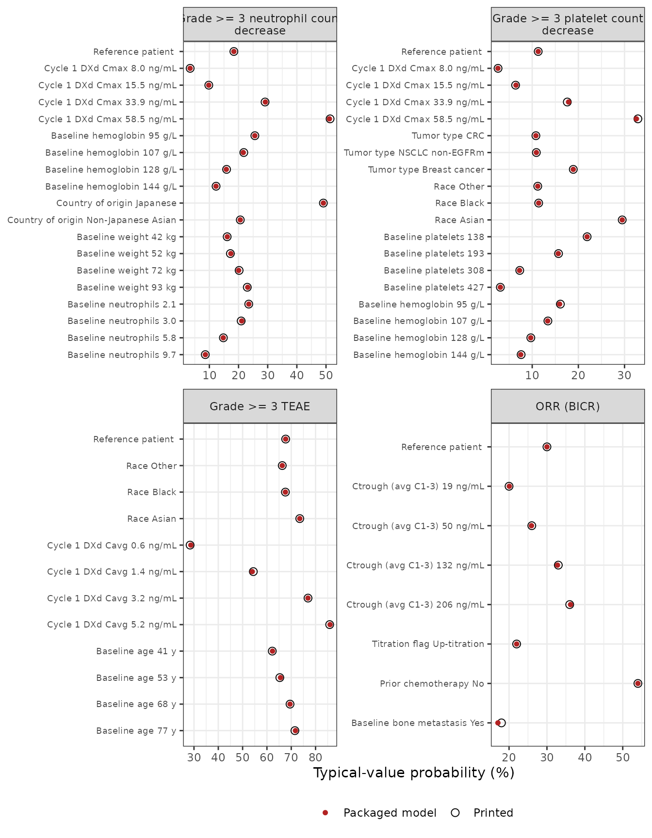
Replicates Figure 2 and Figures S3A, S3B and S4 of Li 2025. Every row matches to within 0.44 percentage points except baseline bone metastasis. That row uses the odds ratio of 0.48 printed in the Results, which gives 17.1% against the forest plot’s 18%. A posterior-median odds ratio and a posterior-median probability need not agree exactly.
Check 2 – an independent ORR statement in the text
The Results state that raising the average Cycle 1-3 trough to 2.25 times the U201 median of 77 ng/mL “would result in a relative increase in ORR by 19.9%”, to a predicted probability of 34.3%. No part of the back-solve used this sentence.
p_orr <- 100 * solve_static("orr", list(list(CTROUGH = 77), list(CTROUGH = 2.25 * 77)))
orr_text <- tibble::tibble(
  Quantity = c("ORR at 2.25 x 77 ng/mL (%)", "Relative increase from 77 ng/mL (%)"),
  Printed = c(34.3, 19.9),
  Model = c(p_orr[2], 100 * (p_orr[2] / p_orr[1] - 1))
)
stopifnot(abs(orr_text$Model[1] - 34.3) < 1.5, abs(orr_text$Model[2] - 19.9) < 3)
knitr::kable(orr_text, digits = 1)| Quantity | Printed | Model |
|---|---|---|
| ORR at 2.25 x 77 ng/mL (%) | 34.3 | 34.9 |
| Relative increase from 77 ng/mL (%) | 19.9 | 20.8 |
The small differences are expected, because the text summarises the posterior distribution of the prediction and the forest plot summarises posterior-median typical values.
Check 3 – the marginal models reproduce Table 4, including a hold-out
Each marginal model is solved at the regimen’s typical exposure: the Table S5 median at 5.6 mg/kg scaled in proportion to dose. The four fixed-dose columns were used to fit the models. The up-titration column was not, so it is a hold-out.
- For the binary endpoints, the Cycle 1 exposure under up-titration is the 3.2 mg/kg exposure.
- For the time-to-event endpoints, the per-cycle exposure follows the 3.2 / 4.8 / 6.4 mg/kg steps.
The time-to-event models are solved over 6 months (182.6 days), with one covariate record per 21-day cycle.
dose_fixed <- c(3.2, 4.8, 5.6, 6.4)
cref <- c(sae = 2.1, nausea_vomiting = 418, ild = 2780, dose_reduction = 24.2,
          discontinuation = 2.1)
covname <- c(sae = "CAV", nausea_vomiting = "CAV", ild = "CMAX", dose_reduction = "CMAX",
             discontinuation = "CAV")
horizon <- 182.625

solve_marginal_binary <- function(suffix, dose) {
  ev <- data.frame(id = seq_along(dose), time = 0, evid = 0L)
  ev[[covname[[suffix]]]] <- cref[[suffix]] * dose / 5.6
  out <- as.data.frame(solve_er(
    mods[[paste0("Li_2025_patritumabDeruxtecan_", suffix)]], events = ev))
  out[[endpoints$output[endpoints$suffix == suffix]]]
}

# One covariate record at the start of each 21-day cycle (LOCF), plus the
# 6-month evaluation time.
tte_events <- function(suffix, cycle_doses, id) {
  starts <- 21 * (seq_along(cycle_doses) - 1)
  ev <- data.frame(id = id, time = c(starts, horizon), evid = 0L)
  ev[[covname[[suffix]]]] <- cref[[suffix]] *
    c(cycle_doses, cycle_doses[length(cycle_doses)]) / 5.6
  ev[order(ev$time), ]
}
solve_marginal_tte <- function(suffix, regimens) {
  ev <- dplyr::bind_rows(lapply(seq_along(regimens), function(k) {
    tte_events(suffix, regimens[[k]], k)
  }))
  out <- as.data.frame(solve_er(
    mods[[paste0("Li_2025_patritumabDeruxtecan_", suffix)]], events = ev))
  out <- out[out$time == horizon, ]
  out[[endpoints$output[endpoints$suffix == suffix]]]
}

ncyc <- ceiling(horizon / 21)
regimens <- c(lapply(dose_fixed, function(d) rep(d, ncyc)),
              list(c(3.2, 4.8, rep(6.4, ncyc - 2))))

table4 <- tibble::tribble(
  ~suffix,            ~`3.2`, ~`4.8`, ~`5.6`, ~`6.4`, ~`Up-titration`,
  "sae",              28,     38,     42,     46,     28,
  "nausea_vomiting",  26,     31,     33,     35,     26,
  "ild",              2.0,    3.7,    4.7,    5.8,    5.3,
  "dose_reduction",   13,     20,     23,     26,     20,
  "discontinuation",  4.7,    7.4,    9.0,    10,     9.3
) |>
  tidyr::pivot_longer(-suffix, names_to = "regimen", values_to = "printed")

sim4 <- dplyr::bind_rows(
  lapply(c("sae", "nausea_vomiting"), function(s) {
    tibble::tibble(suffix = s, regimen = c("3.2", "4.8", "5.6", "6.4", "Up-titration"),
                   simulated = 100 * solve_marginal_binary(s, c(dose_fixed, 3.2)))
  }),
  lapply(c("ild", "dose_reduction", "discontinuation"), function(s) {
    tibble::tibble(suffix = s, regimen = c("3.2", "4.8", "5.6", "6.4", "Up-titration"),
                   simulated = 100 * solve_marginal_tte(s, regimens))
  })
)
check4 <- dplyr::left_join(table4, sim4, by = c("suffix", "regimen")) |>
  dplyr::mutate(diff = simulated - printed)

fixed_rows <- check4$regimen != "Up-titration"
holdout <- check4[!fixed_rows, ]
stopifnot(
  # Fit rows: deterministic back-solve, rounding error only.
  max(abs(check4$diff[fixed_rows])) < 0.35,
  # Hold-outs that pass: SAE and nausea/vomiting exactly, ILD and
  # discontinuation within 0.3 percentage points.
  max(abs(holdout$diff[holdout$suffix != "dose_reduction"])) < 0.3,
  # The documented dose-reduction hold-out failure (24% vs 20%).
  abs(holdout$simulated[holdout$suffix == "dose_reduction"] - 24.0) < 0.2
)

check4 |>
  dplyr::left_join(dplyr::select(endpoints, suffix, endpoint), by = "suffix") |>
  dplyr::mutate(cell = sprintf("%.1f (%.1f)", simulated, printed)) |>
  dplyr::select(endpoint, regimen, cell) |>
  tidyr::pivot_wider(names_from = regimen, values_from = cell) |>
  dplyr::rename(Endpoint = endpoint, `3.2 mg/kg` = `3.2`, `4.8 mg/kg` = `4.8`,
                `5.6 mg/kg` = `5.6`, `6.4 mg/kg` = `6.4`) |>
  knitr::kable(caption = paste(
    "Packaged marginal model (Li 2025 Table 4 in parentheses), %. The",
    "time-to-event endpoints are cumulative probabilities at 6 months. The",
    "up-titration column is a hold-out."
))| Endpoint | 3.2 mg/kg | 4.8 mg/kg | 5.6 mg/kg | 6.4 mg/kg | Up-titration |
|---|---|---|---|---|---|
| SAE | 28.0 (28.0) | 38.0 (38.0) | 42.2 (42.0) | 45.9 (46.0) | 28.0 (28.0) |
| Grade >= 2 nausea or vomiting | 26.0 (26.0) | 31.0 (31.0) | 33.1 (33.0) | 34.9 (35.0) | 26.0 (26.0) |
| Adjudicated drug-related ILD (6 months) | 2.0 (2.0) | 3.7 (3.7) | 4.7 (4.7) | 5.8 (5.8) | 5.1 (5.3) |
| AE leading to dose reduction (6 months) | 13.1 (13.0) | 19.8 (20.0) | 23.0 (23.0) | 26.1 (26.0) | 24.0 (20.0) |
| AE leading to discontinuation (6 months) | 4.8 (4.7) | 7.4 (7.4) | 8.8 (9.0) | 10.1 (10.0) | 9.2 (9.3) |
The dose-reduction hold-out fails: the model gives 24% for
up-titration, where Table 4 prints 20%. Dose reductions are front-loaded
(median onset day 23, Table S4), so the unreported cycle random effects
alpha_j carry weight. A constant per-cycle hazard spreads
the risk evenly and so overstates it under the high later doses of
up-titration. ILD and discontinuation occur later (median onset days 124
and 94), and their hold-outs pass.
Figure 3 – 5.6 mg/kg Q3W versus up-titration
Figure 3 of Li 2025 plots the 5.6 mg/kg and up-titration columns of Table 4. The packaged models are evaluated as follows.
- The five marginal models use the dose-scaled exposures of Check 3.
- The four conditional models are evaluated at the reference patient, using the regimen’s printed median exposure (Table S2 for ORR, Table S5 otherwise). For ORR, the titration flag is also set for up-titration.
typ <- tibble::tribble(
  ~suffix,         ~regimen,        ~set,
  "orr",           "5.6 mg/kg Q3W", list(CTROUGH = 90.9),
  "orr",           "Up-titration",  list(CTROUGH = 58.4, REGIMEN_UPTITRATION = 1),
  "teae_grade3",   "5.6 mg/kg Q3W", list(CAV = 2.1),
  "teae_grade3",   "Up-titration",  list(CAV = 1.1),
  "plt_decrease",  "5.6 mg/kg Q3W", list(CMAX = 24.2),
  "plt_decrease",  "Up-titration",  list(CMAX = 13.0),
  "anc_decrease",  "5.6 mg/kg Q3W", list(CMAX = 24.2),
  "anc_decrease",  "Up-titration",  list(CMAX = 13.0)
)
typ$simulated <- NA_real_
for (s in unique(typ$suffix)) {
  i <- typ$suffix == s
  typ$simulated[i] <- 100 * solve_static(s, typ$set[i])
}
fig3 <- dplyr::bind_rows(
  dplyr::select(typ, suffix, regimen, simulated),
  check4 |>
    dplyr::filter(regimen %in% c("5.6", "Up-titration")) |>
    dplyr::mutate(regimen = ifelse(regimen == "5.6", "5.6 mg/kg Q3W", "Up-titration")) |>
    dplyr::select(suffix, regimen, simulated)
) |>
  dplyr::left_join(
    tibble::tribble(
      ~suffix,           ~`5.6 mg/kg Q3W`, ~`Up-titration`,
      "orr",             33,               24,
      "teae_grade3",     68,               50,
      "sae",             42,               28,
      "plt_decrease",    24,               12,
      "anc_decrease",    27,               14,
      "nausea_vomiting", 33,               26,
      "ild",             4.7,              5.3,
      "dose_reduction",  23,               20,
      "discontinuation", 9.0,              9.3
    ) |>
      tidyr::pivot_longer(-suffix, names_to = "regimen", values_to = "printed"),
    by = c("suffix", "regimen")
  ) |>
  dplyr::left_join(dplyr::select(endpoints, suffix, endpoint, kind), by = "suffix") |>
  dplyr::mutate(endpoint = factor(endpoint, levels = endpoints$endpoint))

ggplot(fig3, aes(x = endpoint, fill = regimen)) +
  geom_col(aes(y = simulated), position = position_dodge(width = 0.8), width = 0.7) +
  geom_point(aes(y = printed, group = regimen), position = position_dodge(width = 0.8),
             shape = 4, size = 2) +
  scale_fill_manual(values = c(`5.6 mg/kg Q3W` = "#1b9e77", `Up-titration` = "#d95f02"),
                    name = NULL) +
  labs(x = NULL, y = "Endpoint probability (%)",
       caption = "Bars: packaged models. Crosses: Li 2025 Table 4 / Figure 3.") +
  theme_bw() +
  theme(axis.text.x = element_text(angle = 35, hjust = 1), legend.position = "top")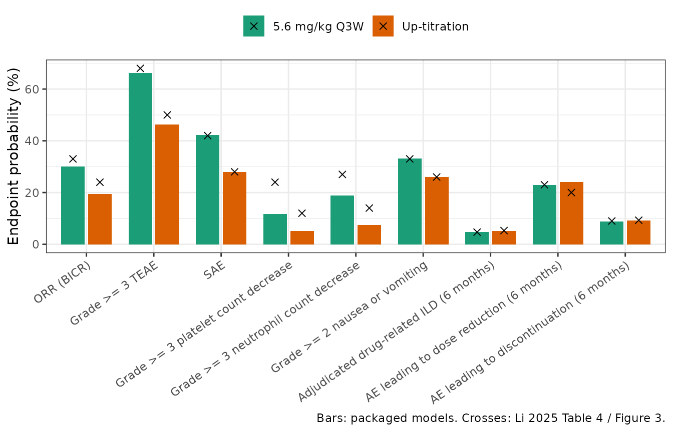
Replicates Figure 3 of Li 2025. The marginal endpoints match by construction, except the dose-reduction hold-out noted above. For the conditional endpoints, the typical-value bars sit below the population-simulated crosses for the safety endpoints, and the next section explains why. The ordering of the two regimens is reproduced for eight of the nine endpoints. The exception is dose reduction, where the failed hold-out places up-titration (24%) above 5.6 mg/kg (23%), while Table 4 places it below (20% vs 23%).
ord <- fig3 |>
  dplyr::select(suffix, regimen, simulated, printed) |>
  tidyr::pivot_wider(names_from = regimen, values_from = c(simulated, printed)) |>
  dplyr::mutate(
    same_order = sign(`simulated_5.6 mg/kg Q3W` - `simulated_Up-titration`) ==
      sign(`printed_5.6 mg/kg Q3W` - `printed_Up-titration`)
  )
stopifnot(identical(ord$suffix[!ord$same_order], "dose_reduction"))
Typical value versus population average
A conditional logistic model evaluated at one typical patient is not
the average over a population. The average of expit() over
a spread of exposures and covariates is pulled towards 50%, and the
Asian, Japanese and low-baseline patients who dominate the NSCLC cohort
sit on the high-risk side of the reference patient. The chunk below
shows the exposure part of this effect for the platelet-decrease model.
It averages the reference patient’s probability over a log-normal Cycle
1 DXd Cmax distribution, using a deterministic grid of 200 quantiles.
The median is the dose-scaled Table S5 median. The log-scale SD is 0.43,
from the Table S5 5.6 mg/kg mean / median ratio,
sqrt(2 * log(26.5 / 24.2)).
sdlog <- sqrt(2 * log(26.5 / 24.2))
q <- (seq_len(200) - 0.5) / 200
pop <- lapply(dose_fixed, function(d) {
  cmax <- stats::qlnorm(q, meanlog = log(24.2 * d / 5.6), sdlog = sdlog)
  p <- solve_static("plt_decrease", lapply(cmax, function(x) list(CMAX = x)))
  tibble::tibble(dose = d,
                 typical = 100 * solve_static("plt_decrease", list(list(CMAX = 24.2 * d / 5.6))),
                 averaged = 100 * mean(p))
}) |>
  dplyr::bind_rows() |>
  dplyr::mutate(`Table 4` = c(12, 20, 24, 28))
stopifnot(all(pop$averaged > pop$typical))
pop |>
  dplyr::rename(`Dose (mg/kg Q3W)` = dose, `Typical patient, median Cmax` = typical,
                `Typical patient, averaged over Cmax` = averaged) |>
  knitr::kable(digits = 1, caption = paste(
    "Grade >= 3 platelet count decrease (%), reference covariates. Averaging",
    "over the exposure spread alone moves the prediction towards Table 4; the",
    "remainder is the covariate mix of the simulated NSCLC population, which",
    "the paper does not print."
))| Dose (mg/kg Q3W) | Typical patient, median Cmax | Typical patient, averaged over Cmax | Table 4 |
|---|---|---|---|
| 3.2 | 5.5 | 6.5 | 12 |
| 4.8 | 9.6 | 10.9 | 20 |
| 5.6 | 11.7 | 13.2 | 24 |
| 6.4 | 13.9 | 15.5 | 28 |
Exposure-response curves
grid <- tibble::tibble(CTROUGH = exp(seq(log(3), log(400), length.out = 100)))
orr_curve <- grid |>
  dplyr::mutate(
    `Fixed dose` = 100 * solve_static("orr", lapply(CTROUGH, function(x) list(CTROUGH = x))),
    `Up-titration` = 100 * solve_static("orr", lapply(CTROUGH, function(x) {
      list(CTROUGH = x, REGIMEN_UPTITRATION = 1)
    }))
  ) |>
  tidyr::pivot_longer(-CTROUGH, names_to = "regimen", values_to = "orr")
ggplot(orr_curve, aes(CTROUGH, orr, colour = regimen)) +
  geom_line(linewidth = 1) +
  geom_vline(xintercept = c(19, 206), linetype = 3) +
  scale_x_log10() +
  labs(x = "Average Cycle 1-3 anti-HER3-ac-DXd Ctrough (ng/mL)",
       y = "Typical-value ORR (%)", colour = NULL,
       caption = "Dotted lines: 5th and 95th exposure percentiles (Figure 2).") +
  theme_bw()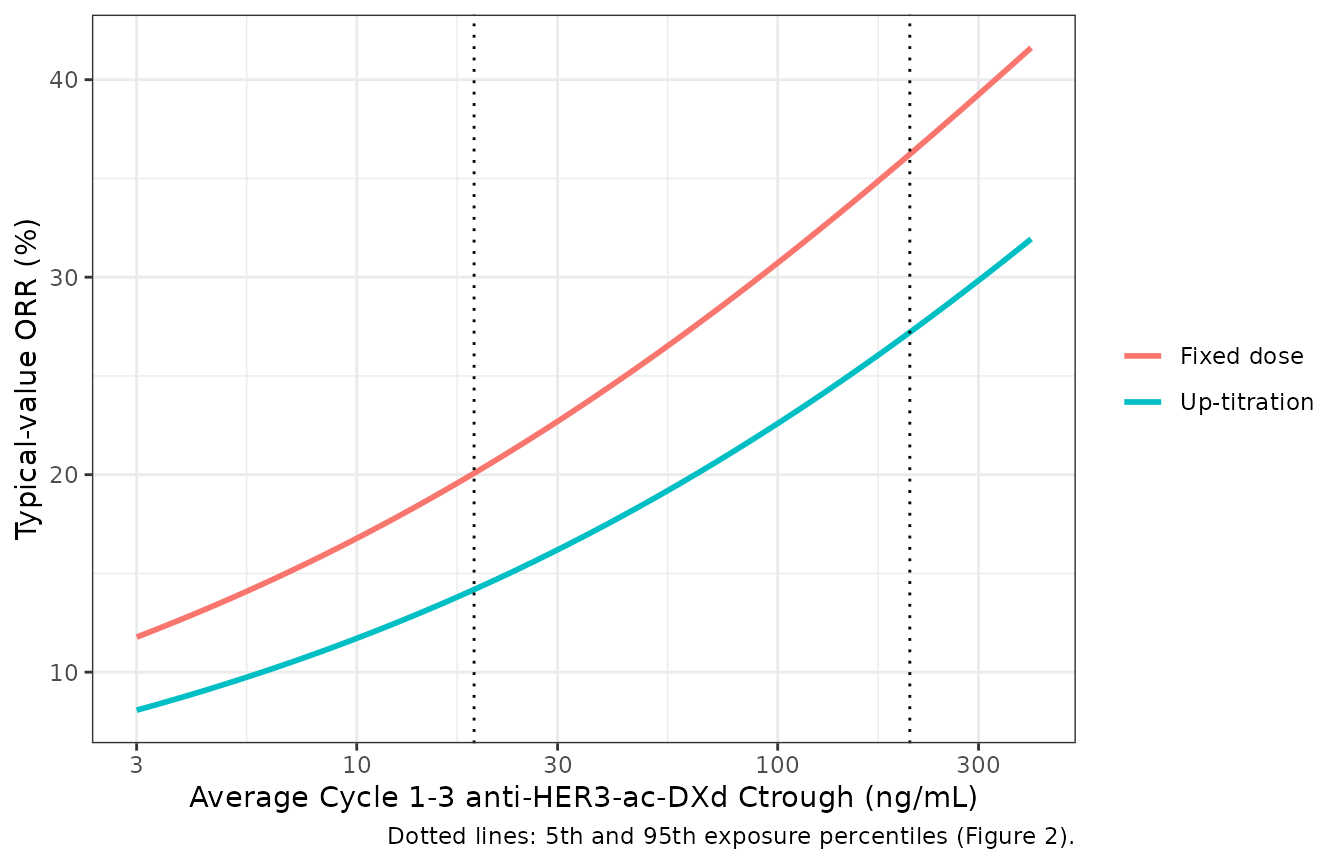
Illustrates the typical-value relationship underlying Figure 1 of Li 2025 (the figure itself is a posterior predictive check against observed response rates, which are not reproducible without the data).
tte_time <- c(lapply(c(3.2, 5.6, 6.4), function(d) rep(d, 18)),
              list(c(3.2, 4.8, rep(6.4, 16))))
reg_lab <- c("3.2 mg/kg Q3W", "5.6 mg/kg Q3W", "6.4 mg/kg Q3W", "Up-titration")
curves <- dplyr::bind_rows(lapply(c("ild", "dose_reduction", "discontinuation"), function(s) {
  ev <- dplyr::bind_rows(lapply(seq_along(tte_time), function(k) {
    starts <- 21 * (seq_along(tte_time[[k]]) - 1)
    e <- data.frame(id = k, time = sort(unique(c(starts, seq(0, 365, by = 3)))), evid = 0L)
    cyc <- pmin(floor(e$time / 21) + 1, length(tte_time[[k]]))
    e[[covname[[s]]]] <- cref[[s]] * tte_time[[k]][cyc] / 5.6
    e
  }))
  out <- as.data.frame(solve_er(mods[[paste0("Li_2025_patritumabDeruxtecan_", s)]],
                                       events = ev))
  tibble::tibble(endpoint = endpoints$endpoint[endpoints$suffix == s],
                 regimen = reg_lab[out$id], time = out$time,
                 prob = 100 * out[[endpoints$output[endpoints$suffix == s]]])
}))
ggplot(curves, aes(time, prob, colour = regimen)) +
  geom_line() +
  geom_vline(xintercept = horizon, linetype = 3) +
  facet_wrap(~endpoint, scales = "free_y", labeller = label_wrap_gen(22)) +
  labs(x = "Time since first dose (days)", y = "Cumulative probability (%)", colour = NULL,
       caption = "Dotted line: 6 months, the time point of Table 4.") +
  theme_bw() +
  theme(legend.position = "bottom")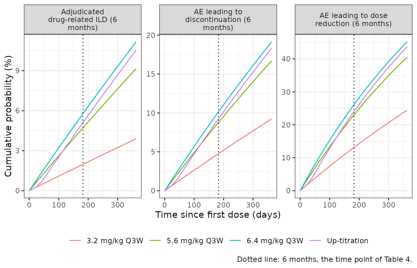
NCA
There is no PK in these models. Every exposure metric is an input
column, so a noncompartmental analysis would only re-measure numbers the
user supplied, and no PKNCA check is included. Users who need the
exposure metrics can compute them from the companion population PK model
(Lee_2023_patritumab).
Assumptions and deviations
- No coefficient is printed in the source. All nine models are reconstructions. They are not the authors’ posterior estimates, and each in-file comment names the figure or table rows the value was solved from.
- Exposure form. The supplement lists linear, log-linear, Emax and sigmoid Emax forms without saying which was chosen for each endpoint. Log-linear is used throughout: it reproduces all four forest plots at rounding precision, where the linear form does not, and it also fits the five Table 4 profiles.
-
Covariate-by-exposure interactions
(
gamma_2in the supplement) cannot be identified from typical-value forest plots, which are evaluated at the reference exposure, and are omitted. - Bone metastasis uses the odds ratio of 0.48 printed in the Results rather than the forest-plot row (17.1% vs 18% at the reference).
-
Reference values.
- Weight (60 kg) and age (61 years) are centred at the printed population medians.
- The reference exposures of the conditional models and the reference platelets (243 x 10^9/L), neutrophils (4.1 x 10^9/L) and hemoglobin (118 g/L) are the values implied by the forest plots, rounded to three significant figures.
- Hemoglobin unit. Figure S3 and Table S1 label hemoglobin “g/dL”, but the values (mean 118, range of percentiles 95-144) are g/L. The models take g/L.
-
Marginal models.
- SAE, nausea / vomiting, ILD, dose reduction and discontinuation are fitted to population-simulated rates. They assume exposure proportional to dose about the Table S5 5.6 mg/kg median.
- They return population-average probabilities, and the influential covariates of the source (age and Japan for SAE, age for dose reduction) are folded into the intercept.
- They are most faithful when given a regimen’s typical exposure, not an individual’s.
-
Time-to-event models.
- The cycle random effects
alpha_j ~ Normal(0, omega)have no printedomegaand are set to zero. - The discrete per-cycle hazard is integrated as a continuous rate over each 21-day cycle, so survival is exact at whole-cycle boundaries and interpolated within a cycle.
- Table 4 is read as 6-month cumulative probabilities, the time point the Results give for ILD and the title of Table S7. Six months is taken as 182.625 days (8.7 cycles).
- The models assume Q3W cycles; the 21-day divisor does not apply to the alternative Q2W regimen.
- The cycle random effects
- Dose reduction fails its up-titration hold-out (24% vs 20%); see Check 3.
- Residual error. The source likelihoods are Bernoulli, with no residual error and no between-subject random effect. Each model carries a fixed placeholder additive residual SD of 0.001 on its probability output, only so that nlmixr2 accepts the model; it is not from the source.
- Duration of response was analysed only by Kaplan-Meier and log-rank test (Figure S1), with no model, so nothing is packaged for it.