Grazoprevir PBPK: saturable OATP1B, CYP3A and P-gp (Yoshikado 2025)
Source:vignettes/articles/Yoshikado_2025_grazoprevir_pbpk.Rmd
Yoshikado_2025_grazoprevir_pbpk.RmdModel and source
- Citation: Yoshikado T, Aoki Y, Nakamura R, Shida S, Sugiyama Y, Chiba K. Elucidating Contributions of Drug Transporters/Enzyme to Nonlinear Pharmacokinetics of Grazoprevir by PBPK Modeling With a Cluster Gauss-Newton Method. CPT Pharmacometrics Syst Pharmacol. 2025;14(4):770-780. doi:10.1002/psp4.13314. The ODE system and the fixed constants not listed in Table S1 (the per-kg organ volumes and blood flows, the gut transit scaling alpha) are transcribed from the authors’ deposited rxode2 model code (Supporting Information R script, reproduced in Data S1 ‘Model equations’). The estimated parameters are the median column of main-text Table 2; the fixed compound and physiological constants are Table S1A.
- Article: https://doi.org/10.1002/psp4.13314 (open access, PMC12001266)
- Supporting Information: Table S1 (fixed and estimated parameter settings), Data S1 (in vitro methods and the model equations) and the authors’ deposited R script, which carries the complete rxode2 model code, the observed data and the CGNM call.
Grazoprevir (GZR), an HCV NS3/4A protease inhibitor, shows strongly more-than-dose-proportional exposure between 50 and 800 mg. It is a substrate of OATP1B1 and OATP1B3 (hepatic uptake), CYP3A (hepatic and intestinal metabolism) and P-gp (biliary excretion and intestinal efflux). Yoshikado et al. fitted a PBPK model of the Sugiyama-laboratory framework – five-unit tandem liver, segregated-flow intestine with duodenum, jejunum and ileum, and enterohepatic circulation – in which all four processes are Michaelis-Menten. They fitted it with the Cluster Gauss-Newton method (CGNM). A first top-down fit (Table 1) reproduced the profiles, but its Km values were unidentifiable or far from the in vitro values. A second, “middle-out” fit added the in vitro Km values as penalised reference values (Equation 2), and gave a tight, identifiable parameter set (Table 2). This package ships that second fit.
Structure
-
Liver: five sinusoidal
(
is_liver1..is_liver5) and five hepatocyte (int_liver1..int_liver5) sub-compartments in series. Uptake is OATP1B1 + OATP1B3 Michaelis-Menten plus passive diffusion on the unbound sinusoidal concentration (fu_b * C); hepatocyte elimination is P-gp biliary excretion plus CYP3A metabolism on the unbound hepatocyte concentration (fu_h * C). - Intestine: stomach -> duodenum -> jejunum -> ileum lumen -> faeces. Each segment has an enterocyte (saturable CYP3A, saturable apical P-gp efflux, passive diffusion) and a mucosal-blood compartment that drains to the liver, plus a serosal tissue compartment.
-
Bile: hepatic P-gp output passes three transit
compartments (
ehc1..ehc3) into the duodenal lumen. - Other tissues: muscle, skin and adipose, perfusion-limited.
-
Pharmacogenomics: the covariate
SNP_SLCO1B1_RS4149056_HOM(c.521 CC) multiplies the OATP1B1 uptake term by 0.344, exactly as the deposited code’s duplicateMT_GZR_*states do.
The model was checked against the deposited code before this vignette was written: for a 100 mg dose, the wild-type and c.521 CC blood profiles, the cumulative faecal excretion and the gut-metabolism integrator agreed to a relative difference below 1e-9 at every time point.
Population
| Field | Value |
|---|---|
| species | human |
| dose_range | single oral doses of 50, 100, 200, 400, 600 and 800 mg |
| disease_state | chronic hepatitis C (genotype 1 and genotype 3 HCV-infected patients) |
| notes | Yoshikado 2025 fits the mean grazoprevir concentration-time profiles of a dose-escalation study (50-800 mg) reported only as a conference abstract (Caro et al., AASLD 2011, MK-5172 in genotype 1 and 3 HCV-infected patients), together with the cumulative faecal excretion of 187 mg from the Zepatier label and the 1.43-fold AUC ratio in SLCO1B1 c.521 CC vs TT subjects (Guo 2019). Subject counts and demographics are not reported. Body weight is fixed at 70 kg because the clinical source does not report it (Table S1A); every organ volume and blood flow in the model is that per-kg value times 70 kg. |
The clinical data are the mean profiles from a dose-escalation study in genotype 1 and 3 HCV-infected patients, reported only as a conference abstract (Caro et al., AASLD 2011). Neither that abstract nor the paper reports subject counts or demographics, and body weight is assumed to be 70 kg (Table S1A). The model has no between-subject variability, so every simulation below is of the single typical subject the paper fitted.
Units and the molecular weight
States hold nmol/L (blood, tissues, lumen) or nmol (stomach, bile, faeces, gut-metabolism integrator), so doses go in as nmol. The deposited event tables convert 1 mg to 1274 nmol (50 mg = 63,700 nmol), i.e. a molecular weight of 784.9 g/mol, the grazoprevir monohydrate. This vignette uses the same factor so that the simulations match the paper’s.
nmol_per_mg <- 1274Source trace
| Item | Value | Source |
|---|---|---|
| beta | 0.658 | Table 2 median |
| CLint,all | 12,900 L/h | Table 2 median |
| fbile | 0.882 | Table 2 median |
| fOATP1B1 | 0.197 | Table 2 median |
| Km,OATP1B1 | 136 nM | Table 2 median |
| Km,OATP1B3 | 0.235 x Km,OATP1B1 = 32.0 nM | Table 2 (footnote a); ratio from deposited code rKm |
| Km,CYP3A | 1570 nM | Table 2 median |
| Km,P-gp | 347 nM | Table 2 median |
| LR | 0.668 | Table 2 median |
| PSdif,ent,BE | 3.86 L/h | Table 2 median |
| Kp,uu | 71.4 | Table 2 median |
| gamma, gamma_ent, AR | 0.24, 0.24, 1 | Table S1A |
| fB, fh, fgut | 0.0241, 0.0173, 0.0197 | Table S1A |
| Kp adipose / gut / muscle / skin | 0.126 / 0.26 / 0.107 / 0.446 | Table S1A |
| RA OATP1B1 mt/wt | 0.344 | Table S1A |
| RA CYP3A, P-gp gut/liver | 0.00741, 0.0365 | Table S1A |
| kbile, kstomach | 0.605, 2.5 1/h | Table S1A |
| kfeces duodenum / jejunum / ileum | 5.12 / 1.47 / 1.21 1/h | Table S1A |
| Fcyp, Fdif (3 segments) | 0.138/0.545/0.317; 0.076/0.395/0.529 | Table S1A |
| Fpgp (3 segments) | 0.057 / 0.273 / 0.670 | Deposited code (Table S1A prints 0.0197 / 0.371 / 0.61) |
| Alpha (transit scaling) | 1 | Deposited code |
| BW | 70 kg | Table S1A |
| Organ volumes and blood flows (per kg) | see model file | Deposited code (Table S1A cites Yoshikado 2016) |
| Rdif = gamma(1-beta)/(Kp,uu - gamma(1-beta)) | - | Deposited code / Data S1 |
| Hepatic uptake, efflux, elimination terms | - | Deposited code / Data S1 (GZR_2 - GZR_11) |
| Intestinal lumen, enterocyte, mucosa ODEs | - | Deposited code / Data S1 (GZR_12 - GZR_14, GZR_21 - GZR_26) |
| SLCO1B1 c.521 CC | OATP1B1 term x 0.344 | Deposited code (MT_GZR states); Methods |
Simulation
# rxode2 warns that a multi-subject solve has no omega; this model has no
# between-subject variability by design, so the warning is not shown.
mod <- readModelDb("Yoshikado_2025_grazoprevir_pbpk")
# The model has no between-subject variability, so the compiled model is
# already the typical-value model (zeroRe() is not needed).
mod_typ <- rxode2::rxode2(mod)

doses <- c(50, 100, 200, 400, 600, 800)
tgrid <- sort(unique(c(seq(0, 4, by = 0.02), seq(4, 24, by = 0.05), seq(24, 168, by = 1))))

make_events <- function(id, dose_mg, times, genotype = 0) {
  data.frame(
    id = id,
    time = c(0, times),
    evid = c(1, rep(0, length(times))),
    amt = c(dose_mg * nmol_per_mg, rep(0, length(times))),
    cmt = c("stomach", rep("central", length(times))),
    dose_mg = dose_mg,
    SNP_SLCO1B1_RS4149056_HOM = genotype
  )
}

ev <- bind_rows(lapply(seq_along(doses), function(i) make_events(i, doses[i], tgrid)))
sim <- rxSolve(mod_typ, ev, keep = "dose_mg", returnType = "data.frame") |>
  mutate(treatment = factor(paste(dose_mg, "mg"), levels = paste(doses, "mg")))
Replicating the published figures
Blood concentration-time profiles (replicates Figure 3B)
The observed points are the mean profiles in the authors’ deposited script.
obs <- bind_rows(
  data.frame(dose_mg = 50, time = c(0.3552, 1.0655, 1.9281, 2.9428, 3.9577, 5.9365, 7.9662, 11.9239, 15.983, 23.797),
             conc = c(1.2951, 3.5889, 10.720, 8.1740, 6.1453, 5.2833, 3.7942, 2.9777, 3.0606, 2.7836)),
  data.frame(dose_mg = 100, time = c(0.6333, 2.2412, 3.0465, 4.0098, 6.0337, 8.1082, 12.1532, 15.9939, 24.0297),
             conc = c(9.7820, 27.135, 38.860, 26.733, 19.162, 13.802, 9.8490, 9.1120, 7.1690)),
  data.frame(dose_mg = 200, time = c(0.6317, 1.0297, 2.0307, 3.0879, 4.0992, 6.0241, 8.0489, 12.0447, 16.0904, 23.8751),
             conc = c(11.725, 23.718, 70.819, 109.34, 99.896, 57.285, 37.587, 23.182, 15.477, 10.117)),
  data.frame(dose_mg = 400, time = c(0.5608, 1.1572, 2.0575, 3.0174, 4.1308, 6.0552, 8.0302, 12.1301, 16.0754, 24.0617),
             conc = c(119.80, 368.70, 1052.3, 1067.5, 864.83, 526.68, 315.97, 138.22, 85.357, 59.228)),
  data.frame(dose_mg = 600, time = c(0.4596, 0.6554, 1.0982, 2.9087, 3.9196, 5.9452, 8.1258, 12.026, 16.0754, 23.862),
             conc = c(121.60, 249.78, 976.85, 2546.9, 2433.4, 1459.9, 584.17, 195.11, 85.357, 45.225)),
  data.frame(dose_mg = 800, time = c(0.7054, 1.0977, 2.0508, 2.9553, 4.0157, 5.9899, 8.1143, 11.9134, 15.9119, 24.0038),
             conc = c(265.19, 1021.8, 2260.3, 3993.1, 4301.1, 2823.3, 2185.2, 729.83, 328.90, 137.08))
) |>
  mutate(treatment = factor(paste(dose_mg, "mg"), levels = paste(doses, "mg")))
ggplot(sim[sim$time > 0 & sim$time <= 24, ], aes(time, Cc)) +
  geom_line(colour = "steelblue") +
  geom_point(data = obs, aes(time, conc)) +
  scale_y_log10() +
  facet_wrap(~treatment, scales = "free_y") +
  labs(x = "Time (h)", y = "Blood grazoprevir (nM)",
       caption = "Replicates Figure 3B of Yoshikado 2025 (line: Table 2 medians; points: observed means).")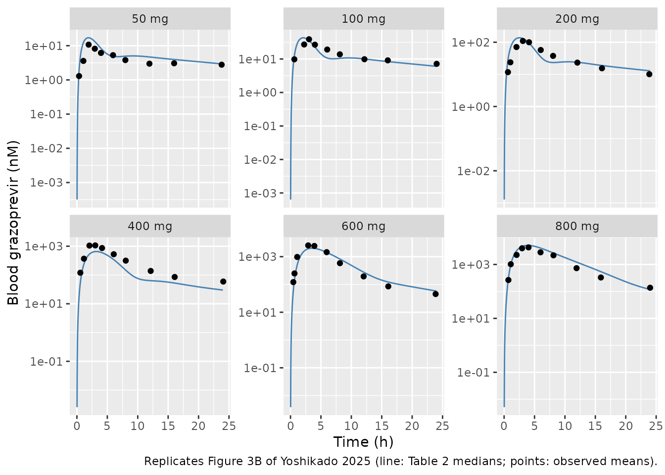
The objective function at the published estimates (Figure 3A)
The middle-out fit minimises SSR’ (Equation 2): the squared log10 residuals of the 59 concentrations, the 187 mg cumulative faecal excretion and the c.521 CC/TT AUC ratio, plus weighted penalties pulling Km,CYP3A, Km,P-gp and Km,OATP1B1 towards 1040, 325 and 170 nM (weights 1.5, 2.2 and 1.6; the weight for Kp,uu is zero). In the deposited script each weight multiplies the log10 value inside the residual, so it enters SSR’ squared. Figure 3A prints a minimum SSR’ of 2.54.
# rxode2 warns that a multi-subject solve has no omega; this model has no
# between-subject variability by design, so the warning is not shown.
# Predictions at the observed sampling times.
ev_obs <- bind_rows(lapply(seq_along(doses), function(i) {
  make_events(i, doses[i], obs$time[obs$dose_mg == doses[i]])
}))
pred_obs <- rxSolve(mod_typ, ev_obs, keep = "dose_mg", returnType = "data.frame")
stopifnot(nrow(pred_obs) == nrow(obs))
res_conc <- log10(obs$conc) - log10(pred_obs$Cc)

# AUC ratio, c.521 CC vs TT, 100 mg, 0-168 h (deposited ID 7).
ev_gen <- bind_rows(make_events(1, 100, 168, 0), make_events(2, 100, 168, 1))
gen <- rxSolve(mod_typ, ev_gen, returnType = "data.frame")
aucr <- gen$auc_blood[gen$id == 2] / gen$auc_blood[gen$id == 1]

# Cumulative faecal excretion, 187 mg, 0-168 h (deposited ID 8).
fec <- rxSolve(mod_typ, make_events(1, 187, 168), returnType = "data.frame")
feces_nmol <- fec$a_feces

theta <- rxode2::rxode2(mod)$theta
km <- exp(theta[c("lkm_cyp3a", "lkm_pgp", "lkm_oatp1b1")])
penalty <- (c(1.5, 2.2, 1.6) * (log10(km) - log10(c(1040, 325, 170))))^2

ssr <- sum(res_conc^2) + (log10(1.43) - log10(aucr))^2 +
  (log10(190589.95) - log10(feces_nmol))^2 + sum(penalty)
knitr::kable(data.frame(
  Component = c("59 blood concentrations", "AUC ratio (c.521 CC/TT)", "Faecal excretion", "Km penalties", "SSR' total"),
  Value = signif(c(sum(res_conc^2), (log10(1.43) - log10(aucr))^2,
                   (log10(190589.95) - log10(feces_nmol))^2, sum(penalty), ssr), 4)
))| Component | Value |
|---|---|
| 59 blood concentrations | 2.367000 |
| AUC ratio (c.521 CC/TT) | 0.000501 |
| Faecal excretion | 0.068980 |
| Km penalties | 0.099940 |
| SSR’ total | 2.537000 |
Faecal excretion and the SLCO1B1 effect (replicates Figure 3C and 3D)
knitr::kable(data.frame(
  Quantity = c("Cumulative faecal GZR, 187 mg, 0-168 h (nmol)", "AUC ratio c.521 CC / TT, 100 mg"),
  Observed = c(190590, 1.43),
  Simulated = signif(c(feces_nmol, aucr), 4)
))| Quantity | Observed | Simulated |
|---|---|---|
| Cumulative faecal GZR, 187 mg, 0-168 h (nmol) | 190590.00 | 1.041e+05 |
| AUC ratio c.521 CC / TT, 100 mg | 1.43 | 1.358e+00 |
stopifnot(
  # Figure 3C: the accepted parameter sets sit near 1e5 nmol, about half the
  # observed amount.
  feces_nmol > 0.4 * 190590, feces_nmol < 0.7 * 190590,
  # Figure 3D: the accepted sets sit just below the observed 1.43.
  aucr > 1.3, aucr < 1.43
)
The model under-predicts the faecal recovery: about 55% of the observed amount. The same gap is visible in the paper’s own Figure 3C, where the accepted parameter sets cluster near 1e5 nmol against an observed 1.9e5 nmol. It is a property of the published fit, not of the transcription.
Saturation of each process (replicates Figure 5)
The Results compare the simulated unbound peak concentration at each site with the corresponding Km (Figure 5):
- sinusoid (
fu_b * is_liver1): exceeds Km,OATP1B3 from 400 mg and Km,OATP1B1 at 800 mg; - hepatocyte (
fu_h * int_liver1): exceeds Km,P-gp from 100 mg and Km,CYP3A from 400 mg; - enterocytes (
fu_gut * <segment>_ent): exceed Km,P-gp at every dose, while for Km,CYP3A “the case varied by the location”.
fu <- c(b = 0.0241, h = 0.0173, gut = 0.0197)
km_all <- c(oatp1b1 = 136, oatp1b3 = 0.235 * 136, cyp3a = 1570, pgp = 347)
peaks <- sim |>
  filter(time <= 24) |>
  group_by(dose_mg) |>
  summarise(
    sinusoid = max(fu[["b"]] * is_liver1),
    hepatocyte = max(fu[["h"]] * int_liver1),
    duodenum = max(fu[["gut"]] * duodenum_ent),
    jejunum = max(fu[["gut"]] * jejunum_ent),
    ileum = max(fu[["gut"]] * ileum_ent),
    .groups = "drop"
  )
knitr::kable(peaks, digits = 1, caption = "Simulated unbound Cmax (nM) by dose")| dose_mg | sinusoid | hepatocyte | duodenum | jejunum | ileum |
|---|---|---|---|---|---|
| 50 | 3.4 | 287.5 | 4728.7 | 1618.5 | 413.8 |
| 100 | 7.4 | 681.2 | 9474.8 | 3245.3 | 831.3 |
| 200 | 16.6 | 1549.8 | 18969.4 | 6501.8 | 1670.4 |
| 400 | 39.9 | 3181.4 | 37960.1 | 13017.2 | 3352.4 |
| 600 | 75.6 | 4765.4 | 56951.3 | 19533.3 | 5036.2 |
| 800 | 148.4 | 6388.2 | 75942.6 | 26049.9 | 6721.0 |
pk <- function(col, dose) peaks[[col]][peaks$dose_mg == dose]
stopifnot(
  pk("sinusoid", 200) < km_all[["oatp1b3"]], pk("sinusoid", 400) > km_all[["oatp1b3"]],
  pk("sinusoid", 600) < km_all[["oatp1b1"]], pk("sinusoid", 800) > km_all[["oatp1b1"]],
  pk("hepatocyte", 50) < km_all[["pgp"]], pk("hepatocyte", 100) > km_all[["pgp"]],
  pk("hepatocyte", 400) > km_all[["cyp3a"]],
  all(unlist(peaks[peaks$dose_mg == 50, c("duodenum", "jejunum", "ileum")]) > km_all[["pgp"]]),
  pk("duodenum", 50) > km_all[["cyp3a"]], pk("ileum", 50) < km_all[["cyp3a"]]
)
Each threshold is crossed at the dose the paper names. At 200 mg the hepatocyte peak (about 1550 nM) sits within 2% of Km,CYP3A, so “exceeds from 400 mg” is the first dose clearly above it.
sim |>
  filter(time > 0, time <= 24) |>
  transmute(time, treatment, Sinusoid = fu[["b"]] * is_liver1, Hepatocyte = fu[["h"]] * int_liver1) |>
  pivot_longer(c(Sinusoid, Hepatocyte), names_to = "site", values_to = "cu") |>
  ggplot(aes(time, cu, colour = treatment)) +
  geom_line() +
  geom_hline(
    data = data.frame(site = c("Sinusoid", "Sinusoid", "Hepatocyte", "Hepatocyte"),
                      km = km_all[c("oatp1b1", "oatp1b3", "cyp3a", "pgp")]),
    aes(yintercept = km), linetype = 2
  ) +
  scale_y_log10() +
  facet_wrap(~site) +
  labs(x = "Time (h)", y = "Unbound GZR (nM)", colour = NULL,
       caption = "Replicates Figure 5A-B of Yoshikado 2025; dashed lines are the Km values.")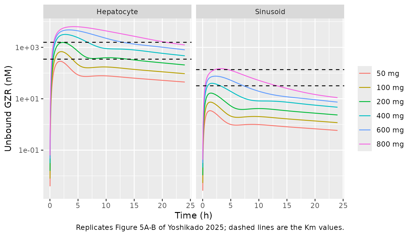
Contribution identities from the Discussion
The Discussion reads three contribution ratios straight off the estimates: OATP1B3 carries about 0.8 of active uptake (1 - fOATP1B1), CYP3A about 0.12 of hepatic elimination (1 - fbile), and in the intestine CYP3A : P-gp = 0.027 : 0.973. The last follows from the fixed gut/liver activity ratios (0.026 from the Table 2 medians; the paper prints 0.027):
th <- theta
cyp_gut <- (1 - th[["f_bile"]]) * th[["vmax_ratio_cyp3a"]]
pgp_gut <- th[["f_bile"]] * th[["vmax_ratio_pgp"]]
ratios <- c(
  oatp1b3 = 1 - th[["f_oatp1b1"]],
  cyp3a_hepatic = 1 - th[["f_bile"]],
  cyp3a_gut = cyp_gut / (cyp_gut + pgp_gut)
)
round(ratios, 3)
#>       oatp1b3 cyp3a_hepatic     cyp3a_gut
#>         0.803         0.118         0.026
stopifnot(abs(ratios[["cyp3a_gut"]] - 0.027) < 0.001)
PKNCA validation
PKNCA is applied to the simulated profiles and, as the reference, to the observed mean profiles of the deposited script (a time-zero concentration of zero is added to each observed profile). Figure S3 reports AUC as the blood-concentration integral from 0 to the last sample (24 h).
# The 0-24 h interval below bounds the AUC; the grid itself runs to 168 h.
sim_nca <- sim |>
  filter(!is.na(Cc)) |>
  select(id, time, Cc, treatment)
dose_df <- sim |>
  filter(time == 0) |>
  distinct(id, treatment) |>
  mutate(time = 0, amt = doses[as.integer(treatment)] * nmol_per_mg)

conc_sim <- PKNCAconc(sim_nca, Cc ~ time | treatment + id)
dose_sim <- PKNCAdose(dose_df, amt ~ time | treatment + id)
intervals <- data.frame(start = 0, end = 24, cmax = TRUE, tmax = TRUE, auclast = TRUE)
nca_sim <- pk.nca(PKNCAdata(conc_sim, dose_sim, intervals = intervals))

obs_nca <- obs |>
  mutate(id = as.integer(treatment)) |>
  bind_rows(data.frame(dose_mg = doses, time = 0, conc = 0,
                       treatment = factor(paste(doses, "mg"), levels = paste(doses, "mg")),
                       id = seq_along(doses))) |>
  arrange(id, time)
conc_obs <- PKNCAconc(obs_nca, conc ~ time | treatment + id)
dose_obs <- PKNCAdose(
  data.frame(treatment = factor(paste(doses, "mg"), levels = paste(doses, "mg")),
             id = seq_along(doses), time = 0, amt = doses * nmol_per_mg),
  amt ~ time | treatment + id
)
nca_obs <- pk.nca(PKNCAdata(conc_obs, dose_obs,
                            intervals = data.frame(start = 0, end = Inf, cmax = TRUE, tmax = TRUE, auclast = TRUE)))

ref <- as.data.frame(nca_obs) |>
  filter(PPTESTCD %in% c("cmax", "tmax", "auclast")) |>
  select(treatment, PPTESTCD, PPORRES) |>
  pivot_wider(names_from = PPTESTCD, values_from = PPORRES)
Comparison against the observed NCA
tbl <- ncaComparisonTable(
  nca_sim, ref,
  by = "treatment",
  params = c("cmax", "tmax", "auclast"),
  units = c(cmax = "nM", tmax = "h", auclast = "nM*h")
)
knitr::kable(tbl)| NCA parameter | treatment | Reference | Simulated | % diff |
|---|---|---|---|---|
| Cmax (nM) | 50 mg | 10.7 | 17 | +58.9%* |
| Cmax (nM) | 100 mg | 38.9 | 43 | +10.7% |
| Cmax (nM) | 200 mg | 109 | 138 | +25.8%* |
| Cmax (nM) | 400 mg | 1070 | 655 | -38.7%* |
| Cmax (nM) | 600 mg | 2550 | 2020 | -20.7%* |
| Cmax (nM) | 800 mg | 4300 | 5090 | +18.4% |
| Tmax (h) | 50 mg | 1.93 | 1.88 | -2.5% |
| Tmax (h) | 100 mg | 3.05 | 2.1 | -31.1%* |
| Tmax (h) | 200 mg | 3.09 | 2.52 | -18.4% |
| Tmax (h) | 400 mg | 3.02 | 3.18 | +5.4% |
| Tmax (h) | 600 mg | 2.91 | 3.56 | +22.4%* |
| Tmax (h) | 800 mg | 4.02 | 3.9 | -2.9% |
| AUClast (nM*h) | 50 mg | 93.7 | 131 | +40.1%* |
| AUClast (nM*h) | 100 mg | 319 | 304 | -5.0% |
| AUClast (nM*h) | 200 mg | 796 | 860 | +8.1% |
| AUClast (nM*h) | 400 mg | 6920 | 4000 | -42.2%* |
| AUClast (nM*h) | 600 mg | 14400 | 13900 | -3.5% |
| AUClast (nM*h) | 800 mg | 30200 | 40000 | +32.5%* |
attr(tbl, "footnote")
#> [1] "* differs from reference by more than ±20%."
The fit captures the roughly 300-fold rise in exposure over a 16-fold dose range (50 to 800 mg):
auc_sim <- as.data.frame(nca_sim) |>
  filter(PPTESTCD == "auclast") |>
  arrange(treatment)
auc_ratio_sim <- auc_sim$PPORRES[auc_sim$treatment == "800 mg"] / auc_sim$PPORRES[auc_sim$treatment == "50 mg"]
auc_ratio_obs <- ref$auclast[ref$treatment == "800 mg"] / ref$auclast[ref$treatment == "50 mg"]
c(simulated = auc_ratio_sim, observed = auc_ratio_obs, dose_ratio = 16)
#>  simulated   observed dose_ratio
#>   304.7086   322.1249    16.0000
stopifnot(auc_ratio_sim > 200, auc_ratio_obs > 200)
The starred rows are deviations of the published fit, not of the transcription. The SSR’ check above reproduces the paper’s own minimum, so the residuals themselves are the paper’s. The largest gaps are at 50 mg, where the model over-predicts a flat, slightly double-peaked observed profile (Figure 3B), and at 400 mg, where it under-predicts the observed peak. The fit balances all six doses on a log10 scale, so it over-predicts some doses and under-predicts others.
Assumptions and deviations
- Estimates are the Table 2 medians. CGNM returns an ensemble of accepted parameter sets and tabulates marginal quantiles; a vector of medians is not itself guaranteed to be an accepted set. Here the ensemble is tight (25th and 75th percentiles agree to three figures), and the median vector gives SSR’ = 2.537, equal to the printed minimum of 2.54.
- Regional P-gp fractions. Table S1A prints Fpgp = 0.0197 / 0.371 / 0.61 (duodenum / jejunum / ileum), while the deposited code uses 0.057 / 0.273 / 0.670. The code is used because it produced Table 2. At the Table 2 medians the two sets give SSR’ of 2.5367 and 2.5364, so the discrepancy does not affect the fit.
- Km,OATP1B3 ratio. The Table 2 footnote gives the OATP1B3/OATP1B1 Km ratio as 0.236; the deposited code uses 0.235, which matches both the in vitro ratio (39.9/170 nM = 0.2347) and the tabulated Km,OATP1B3 of 32.0 nM (0.235 x 136). The code value is used.
-
Unlisted constants. The organ volumes and blood
flows (L/kg, L/h/kg), the transit scaling
alpha(= 1) and the renal clearance (= 0) are not tabulated in the paper beyond a citation of the framework paper. They are the coefficients written in the deposited code. -
Blood vs plasma. The model’s central compartment
and the paper’s figures are whole-blood concentrations. Table S1A lists
a blood-to-plasma ratio of 0.67, but the model equations never use it,
and the paper does not say whether the observed plasma means were
converted to blood before fitting. A plasma concentration can be
approximated as
Cc / 0.67. -
Genotype covariate. The paper simulates the c.521
CC subject with a duplicate set of states in which only the OATP1B1
uptake term is scaled by 0.344; the covariate
SNP_SLCO1B1_RS4149056_HOMreproduces this exactly. Heterozygotes are not modelled; with the indicator at 0 a subject is wild type. -
No variability and a placeholder residual error.
CGNM is a fixed-effects least-squares method. The model has no
between-subject variability, and
propSd = 0.10is a placeholder required for a valid nlmixr2 model, not an estimate. -
Body weight. Every volume and flow scales with the
fixed
bw = 70kg; the clearance-type estimates (CLint,all, PSdif,ent,BE) are absolute (L/h). Changingbwalone therefore does not give a physiologically consistent scaled individual, and the model carries no weight covariate. - Top-down fit not shipped. The top-down analysis (Table 1) was the paper’s first step. Its Km,CYP3A and Km,P-gp are unidentifiable (their 25th-75th percentile ranges span many orders of magnitude), and the paper supersedes it with the middle-out fit.