Model and source
- Citation: Chen X, Wang D, Zhu L, Lu J, Huang Y, Wang G, Zhu Y, Ye Q, Wang Y, Xu H, Li Z. Population Pharmacokinetics and Initial Dose Optimization of Sirolimus Improving Drug Blood Level for Seizure Control in Pediatric Patients With Tuberous Sclerosis Complex. Front Pharmacol. 2021;12:647232. doi:10.3389/fphar.2021.647232.
- Description: One-compartment population PK model with first-order absorption for oral sirolimus whole-blood trough concentrations in Chinese pediatric patients with tuberous sclerosis complex (TSC)-related epilepsy (Chen 2021). The absorption rate constant ka is fixed at 0.485 1/h from the literature because only trough concentrations were available. Apparent oral clearance CL/F is allometrically scaled by body weight (fixed exponent 0.75, reference 70 kg) and multiplied by 1.16 with concomitant oxcarbazepine (power form 1.16^CONMED_OXC). Apparent volume V/F is scaled linearly by body weight (fixed exponent 1). Exponential IIV on CL/F only; additive residual error.
- Article: https://doi.org/10.3389/fphar.2021.647232 (open access, PMC8114543)
Chen et al. (2021) fitted a one-compartment model with first-order absorption to routine therapeutic-drug-monitoring trough concentrations of oral sirolimus in children with tuberous sclerosis complex (TSC)-related epilepsy, and used Monte Carlo simulation to recommend weight-banded initial doses that reach the 5-10 ng/mL trough window associated with seizure control. Because only troughs were available, the absorption rate constant was fixed at 0.485 1/h from the group’s earlier sirolimus model (Wang 2020, cited in the Methods).
Population
Eighty Chinese children (35 boys, 45 girls) treated at the Children’s Hospital of Fudan University between May 2016 and October 2020 contributed 188 whole-blood trough concentrations (2.35 per patient, Emit 2000 assay, linear range 3.5-30 ng/mL). From Table 1: age median 5.76 (range 0.61-16.61) years, weight median 20.50 (8.00-68.00) kg. Sirolimus was given once daily as tablet or oral solution (41 person-times each). Co-medications were valproic acid (40), oxcarbazepine (23), vigabatrin (12), levetiracetam (10), topiramate (8), lamotrigine (4) and carbamazepine (2); only oxcarbazepine was retained, on CL/F.
Source trace
| Element | Value | Source |
|---|---|---|
| Structure: 1-compartment, first-order absorption and elimination | – | Methods, Population Pharmacokinetic Model |
lka |
0.485 1/h (fixed) | Table 2; Methods (Wang 2020) |
lcl |
8.59 L/h | Table 2; Results Eq. 8 |
lvc |
294 L | Table 2; Results Eq. 9 |
e_wt_cl |
0.75 (fixed), reference 70 kg | Methods Eq. 5; Results Eq. 8 |
e_wt_vc |
1 (fixed), reference 70 kg | Methods Eq. 5; Results Eq. 9 |
e_oxc_cl |
1.16, power form 1.16^OXC
|
Table 2 (theta OXC); Methods Eq. 7; Results Eq. 8 |
etalcl |
0.175^2 = 0.030625 | Table 2 (omega CL/F = 0.175, read as SD; see below) |
Exponential IIV P = TV * exp(eta), none on V/F |
– | Methods Eq. 1; Results, Evaluation |
addSd |
1.913 ng/mL | Table 2 (sigma 1, additive); Methods Eq. 2 |
Virtual cohort and simulation
Figures 2-5 simulate 1,000 virtual children at each of eight body weights (5, 10, 20, 30, 40, 50, 60 and 70 kg) and ten daily doses (0.01-0.10 mg/kg/day) under four scenarios (once or twice daily, with or without oxcarbazepine), and print under each dose the probability that the trough lies in the 5-10 ng/mL window. Figure 6 plots the same probabilities against weight.
We simulate 200 children per weight-by-scenario arm (the package cap)
for 14 days and read the trough at the end of the last dosing interval
(336 h). The twice-daily regimen splits the daily dose evenly into two
doses 12 h apart. The model is linear, and Cc is the
individual prediction without residual error, so each child is simulated
once at 0.01 mg/kg/day and the trough at the other nine doses is that
trough multiplied by the dose ratio.
mod <- readModelDb("Chen_2021_sirolimus")

weights <- c(5, 10, 20, 30, 40, 50, 60, 70)
nsub <- 200
ndays <- 14
ref_dose <- 0.01 # mg/kg/day

scenarios <- tibble::tribble(
  ~scenario,          ~CONMED_OXC, ~per_day, ~figure,
  "Once daily",        0,          1,        "Figure 2",
  "Twice daily",       0,          2,        "Figure 3",
  "Once daily + OXC",  1,          1,        "Figure 4",
  "Twice daily + OXC", 1,          2,        "Figure 5"
)

make_arm <- function(sc, wt, id0) {
  ids <- id0 + seq_len(nsub)
  tau <- 24 / sc$per_day
  dtimes <- seq(0, by = tau, length.out = ndays * sc$per_day)
  dose <- tidyr::expand_grid(id = ids, time = dtimes) |>
    mutate(amt = ref_dose * wt / sc$per_day, evid = 1L, cmt = "depot")
  obs <- tibble(id = ids, time = ndays * 24, amt = 0, evid = 0L, cmt = "central")
  bind_rows(dose, obs) |>
    mutate(WT = wt, CONMED_OXC = sc$CONMED_OXC, scenario = sc$scenario)
}

arms <- list()
id0 <- 0
for (i in seq_len(nrow(scenarios))) {
  for (wt in weights) {
    arms[[length(arms) + 1]] <- make_arm(scenarios[i, ], wt, id0)
    id0 <- id0 + nsub
  }
}
ev <- bind_rows(arms) |> arrange(id, time, desc(evid))

rxode2::rxSetSeed(2021)
sim <- rxode2::rxSolve(mod, events = ev, keep = c("WT", "scenario"))
#> ℹ parameter labels from comments will be replaced by 'label()'
trough <- as.data.frame(sim) |>
  filter(time == ndays * 24) |>
  select(id, WT, scenario, Cc)

pta <- tidyr::expand_grid(trough, dose = round(seq(0.01, 0.10, by = 0.01), 2)) |>
  mutate(Ctrough = Cc * dose / ref_dose) |>
  group_by(scenario, WT, dose) |>
  summarise(
    sim_pta = 100 * mean(Ctrough >= 5 & Ctrough <= 10),
    sim_med = median(Ctrough),
    .groups = "drop"
  )
The percentages printed under panels A-F (5-50 kg) of Figures 2-5 are transcribed below. Panels G and H (60 and 70 kg) have labels that are partly hidden by the scatter and are not used in the comparison.
pub_vals <- list(
  "Once daily" = list(
    `5` = c(0, 0, 1.9, 15.0, 42.0, 64.0, 76.7, 77.8, 69.2, 56.1),
    `10` = c(0, 0, 12.5, 48.9, 77.5, 81.2, 68.4, 50.8, 34.3, 19.6),
    `20` = c(0, 3.5, 45.0, 82.0, 79.2, 54.9, 32.2, 14.7, 6.6, 3.1),
    `30` = c(0, 9.7, 66.7, 85.9, 62.1, 33.2, 13.6, 4.6, 2.0, 0.5),
    `40` = c(0, 17.8, 81.2, 80.2, 46.3, 17.5, 5.7, 2.1, 0.3, 0),
    `50` = c(0, 27.7, 86.0, 71.9, 34.1, 11.2, 3.1, 0.5, 0, 0)
  ),
  "Twice daily" = list(
    `5` = c(0, 0, 20.3, 71.6, 90.0, 79.3, 53.8, 28.8, 13.3, 6.5),
    `10` = c(0, 1.6, 53.1, 91.4, 80.0, 47.3, 18.3, 7.0, 2.2, 0.4),
    `20` = c(0, 11.7, 86.3, 88.1, 48.2, 13.7, 4.2, 0.5, 0, 0),
    `30` = c(0, 25.1, 94.3, 75.2, 25.6, 5.8, 0.5, 0, 0, 0),
    `40` = c(0, 38.4, 97.0, 62.1, 14.4, 2.4, 0.1, 0, 0, 0),
    `50` = c(0, 49.7, 97.5, 50.6, 9.1, 0.5, 0, 0, 0, 0)
  ),
  "Once daily + OXC" = list(
    `5` = c(0, 0, 0, 3.6, 14.0, 31.4, 50.8, 64.3, 74.2, 73.6),
    `10` = c(0, 0, 3.0, 18.1, 47.1, 69.5, 77.8, 76.2, 66.1, 51.5),
    `20` = c(0, 0.2, 15.7, 55.3, 79.7, 79.7, 63.9, 44.4, 27.6, 16.1),
    `30` = c(0, 1.8, 33.2, 76.5, 82.8, 66.0, 42.5, 21.9, 12.0, 5.3),
    `40` = c(0, 4.3, 49.6, 83.0, 76.5, 50.5, 25.4, 12.7, 4.8, 2.3),
    `50` = c(0, 8.1, 63.1, 86.0, 67.8, 37.4, 16.1, 6.2, 2.4, 0.7)
  ),
  "Twice daily + OXC" = list(
    `5` = c(0, 0, 5.6, 39.1, 77.1, 87.4, 79.6, 61.0, 40.4, 23.0),
    `10` = c(0, 0, 24.1, 76.0, 89.1, 75.6, 49.3, 24.2, 11.5, 5.4),
    `20` = c(0, 2.0, 59.2, 92.5, 76.5, 41.4, 15.3, 5.6, 1.3, 0.2),
    `30` = c(0, 7.5, 79.6, 91.3, 57.2, 20.6, 6.3, 1.2, 0.1, 0),
    `40` = c(0, 14.1, 88.5, 85.8, 42.2, 11.6, 2.9, 0.3, 0, 0),
    `50` = c(0, 22.0, 93.0, 78.1, 29.8, 7.0, 0.8, 0.1, 0, 0)
  )
)
published <- lapply(names(pub_vals), function(sc) {
  lapply(names(pub_vals[[sc]]), function(wt) {
    tibble(
      scenario = sc, WT = as.numeric(wt), dose = round(seq(0.01, 0.10, by = 0.01), 2),
      pub_pta = pub_vals[[sc]][[wt]]
    )
  }) |>
    bind_rows()
}) |>
  bind_rows()

cmp <- inner_join(published, pta, by = c("scenario", "WT", "dose")) |>
  mutate(diff_pp = sim_pta - pub_pta)
cmp |>
  group_by(scenario) |>
  summarise(
    n_cells = n(),
    median_diff = median(diff_pp),
    median_abs_diff = median(abs(diff_pp)),
    p90_abs_diff = quantile(abs(diff_pp), 0.9),
    .groups = "drop"
  ) |>
  left_join(select(scenarios, scenario, figure), by = "scenario") |>
  select(figure, scenario, n_cells, median_diff, median_abs_diff, p90_abs_diff) |>
  dplyr::rename(
    "Source" = figure, "Scenario" = scenario, "Weight x dose cells" = n_cells,
    "Median difference (pp)" = median_diff,
    "Median |difference| (pp)" = median_abs_diff,
    "90th percentile |difference| (pp)" = p90_abs_diff
  ) |>
knitr::kable(digits = 1, caption = "Simulated minus published probability of a 5-10 ng/mL trough (percentage points), panels A-F of Figures 2-5.")| Source | Scenario | Weight x dose cells | Median difference (pp) | Median |difference| (pp) | 90th percentile |difference| (pp) |
|---|---|---|---|---|---|
| Figure 2 | Once daily | 60 | 0 | 1.3 | 4.2 |
| Figure 4 | Once daily + OXC | 60 | 0 | 1.6 | 4.4 |
| Figure 3 | Twice daily | 60 | 0 | 0.8 | 9.4 |
| Figure 5 | Twice daily + OXC | 60 | 0 | 1.3 | 6.8 |
# The probability of target attainment moves by tens of percentage points
# when a typical value, the allometric reference, the oxcarbazepine factor or
# the IIV scale is wrong (reading omega as a variance lowers the 80-90%
# plateaus to about 40%). Monte Carlo noise at 200 children per arm is about
# 3.5 pp at a 50% probability, so the envelope check uses the 90th percentile
# of |difference| rather than the maximum. Cells where both sides are near 0%
# or 100% carry no information, so the centre and envelope are computed over
# the cells with a published probability between 5% and 95%.
informative <- filter(cmp, pub_pta > 5, pub_pta < 95)
stopifnot(
  nrow(informative) > 100,
  abs(median(informative$diff_pp)) < 3,
  quantile(abs(informative$diff_pp), 0.9) < 10
)
pta |>
  mutate(dose = factor(sprintf("%.2f", dose))) |>
  ggplot(aes(WT, sim_pta, colour = dose)) +
  geom_line() +
  geom_point(
    data = cmp |> mutate(dose = factor(sprintf("%.2f", dose))),
    aes(y = pub_pta), size = 1.2
  ) +
  facet_wrap(~ factor(scenario, levels = scenarios$scenario)) +
  labs(
    x = "Body weight (kg)", y = "Probability of 5-10 ng/mL trough (%)",
    colour = "Dose (mg/kg/day)"
  )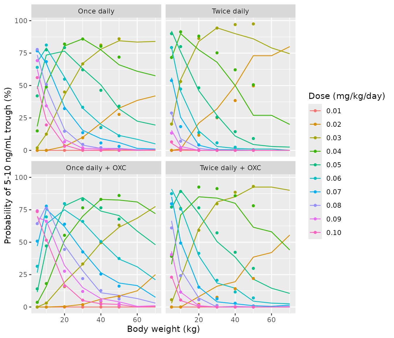
Simulated probability of a 5-10 ng/mL trough against body weight, by daily dose (lines), with the percentages printed in Figures 2-5 (points). Replicates Figure 6 of Chen 2021.
tidyr::expand_grid(filter(trough, scenario == "Once daily", WT == 20), dose = round(seq(0.01, 0.10, by = 0.01), 2)) |>
  mutate(Ctrough = Cc * dose / ref_dose) |>
  ggplot(aes(factor(sprintf("%.2f", dose)), Ctrough)) +
  geom_jitter(width = 0.3, size = 0.5, alpha = 0.5) +
  geom_hline(yintercept = c(5, 10), linetype = "dashed", colour = "red") +
  labs(x = "Dose (mg/kg/day)", y = "Trough sirolimus (ng/mL)")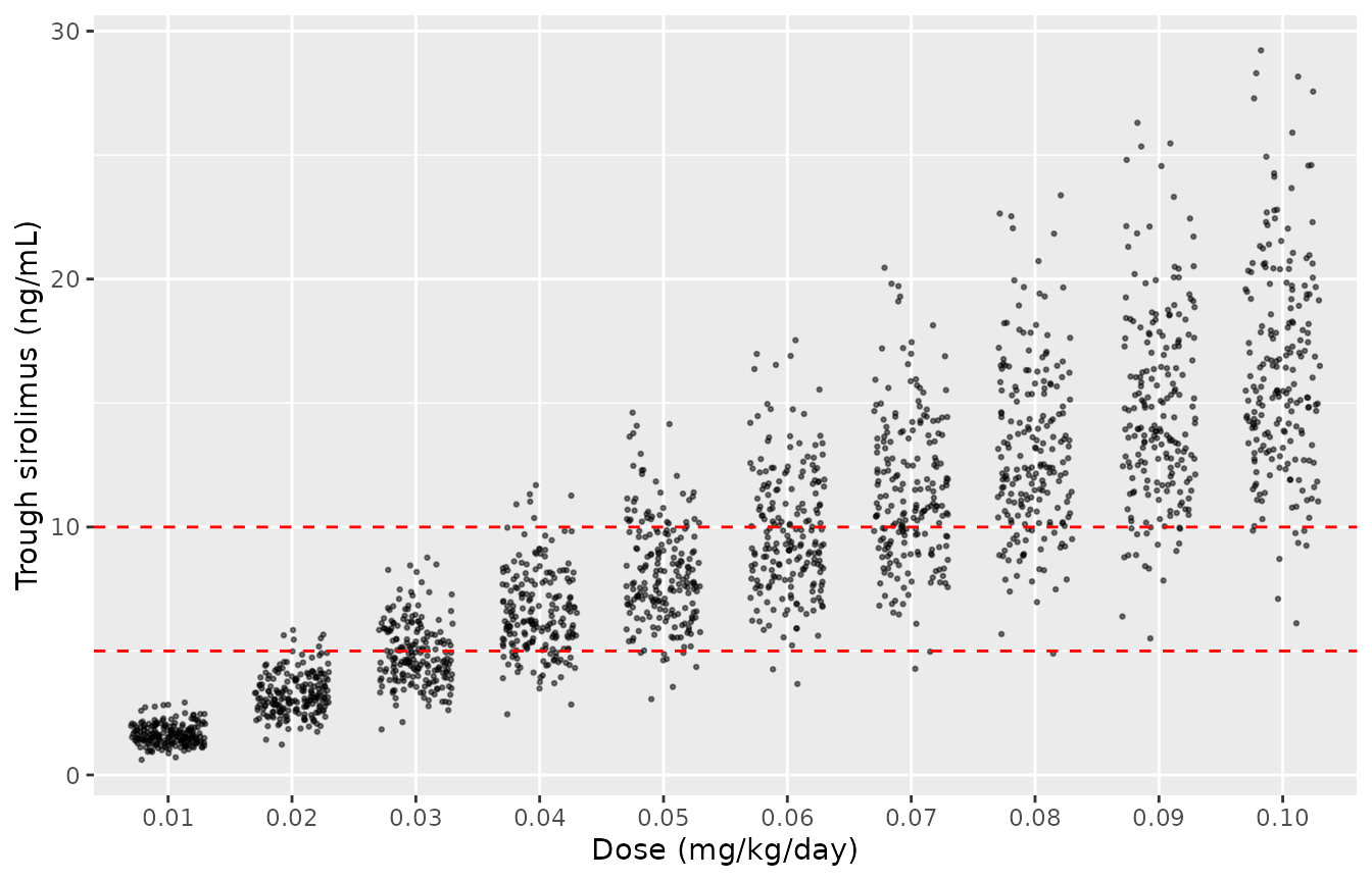
Simulated steady-state trough concentrations by dose at 20 kg, once daily without oxcarbazepine (200 children per dose). Dashed lines: 5-10 ng/mL window. Replicates Figure 2C of Chen 2021.
Initial dose recommendations (Table 3)
Table 3 gives the dose recommended for each weight band. The simulated probability of reaching the window at each simulated weight with the Table 3 dose is shown below; the band edges in Table 3 are where the Figure 6 curves cross, so a weight at a band edge sits between two nearly equal doses.
table3 <- tibble::tribble(
  ~scenario,          ~lo,  ~hi,  ~dose,
  "Once daily",        5,    7.5,  0.07,
  "Once daily",        7.5,  11.5, 0.06,
  "Once daily",        11.5, 19,   0.05,
  "Once daily",        19,   40,   0.04,
  "Once daily",        40,   70,   0.03,
  "Twice daily",       5,    8,    0.05,
  "Twice daily",       8,    20,   0.04,
  "Twice daily",       20,   70,   0.03,
  "Once daily + OXC",  5,    7.5,  0.09,
  "Once daily + OXC",  7.5,  10,   0.08,
  "Once daily + OXC",  10,   13.5, 0.07,
  "Once daily + OXC",  13.5, 20,   0.06,
  "Once daily + OXC",  20,   35,   0.05,
  "Once daily + OXC",  35,   70,   0.04,
  "Twice daily + OXC", 5,    7,    0.06,
  "Twice daily + OXC", 7,    14.5, 0.05,
  "Twice daily + OXC", 14.5, 38,   0.04,
  "Twice daily + OXC", 38,   70,   0.03
)

rec <- tidyr::expand_grid(scenario = scenarios$scenario, WT = weights) |>
  rowwise() |>
  mutate(rec_dose = {
    rows <- table3[table3$scenario == scenario & WT >= table3$lo & WT <= table3$hi, ]
    rows$dose[1]
  }) |>
  ungroup() |>
  left_join(pta, by = c("scenario", "WT", "rec_dose" = "dose")) |>
  group_by(scenario, WT) |>
  mutate(
    best_dose = pta$dose[pta$scenario == scenario[1] & pta$WT == WT[1]][
      which.max(pta$sim_pta[pta$scenario == scenario[1] & pta$WT == WT[1]])
    ]
  ) |>
  ungroup()

rec |>
  select(scenario, WT, rec_dose, sim_pta, sim_med, best_dose) |>
  dplyr::rename(
    "Scenario" = scenario, "Weight (kg)" = WT,
    "Table 3 dose (mg/kg/day)" = rec_dose,
    "Simulated P(5-10 ng/mL) (%)" = sim_pta,
    "Simulated median trough (ng/mL)" = sim_med,
    "Simulated best dose (mg/kg/day)" = best_dose
  ) |>
knitr::kable(digits = 2, caption = "Table 3 recommendations evaluated with the model.")| Scenario | Weight (kg) | Table 3 dose (mg/kg/day) | Simulated P(5-10 ng/mL) (%) | Simulated median trough (ng/mL) | Simulated best dose (mg/kg/day) |
|---|---|---|---|---|---|
| Once daily | 5 | 0.07 | 77.5 | 6.84 | 0.07 |
| Once daily | 10 | 0.06 | 79.0 | 7.65 | 0.06 |
| Once daily | 20 | 0.04 | 80.5 | 6.20 | 0.04 |
| Once daily | 30 | 0.04 | 86.0 | 7.38 | 0.04 |
| Once daily | 40 | 0.04 | 77.5 | 7.96 | 0.03 |
| Once daily | 50 | 0.03 | 84.5 | 6.70 | 0.03 |
| Once daily | 60 | 0.03 | 83.5 | 7.01 | 0.03 |
| Once daily | 70 | 0.03 | 84.0 | 7.29 | 0.03 |
| Twice daily | 5 | 0.05 | 92.0 | 6.93 | 0.05 |
| Twice daily | 10 | 0.04 | 90.0 | 6.91 | 0.04 |
| Twice daily | 20 | 0.04 | 77.5 | 8.16 | 0.03 |
| Twice daily | 30 | 0.03 | 94.5 | 6.90 | 0.03 |
| Twice daily | 40 | 0.03 | 90.0 | 7.50 | 0.03 |
| Twice daily | 50 | 0.03 | 86.0 | 8.24 | 0.03 |
| Twice daily | 60 | 0.03 | 79.0 | 8.55 | 0.03 |
| Twice daily | 70 | 0.03 | 74.5 | 8.90 | 0.02 |
| Once daily + OXC | 5 | 0.09 | 69.0 | 6.36 | 0.10 |
| Once daily + OXC | 10 | 0.08 | 78.0 | 7.72 | 0.08 |
| Once daily + OXC | 20 | 0.06 | 75.0 | 7.79 | 0.05 |
| Once daily + OXC | 30 | 0.05 | 84.5 | 7.60 | 0.05 |
| Once daily + OXC | 40 | 0.04 | 83.0 | 6.65 | 0.04 |
| Once daily + OXC | 50 | 0.04 | 82.5 | 7.09 | 0.04 |
| Once daily + OXC | 60 | 0.04 | 81.0 | 7.62 | 0.04 |
| Once daily + OXC | 70 | 0.04 | 72.0 | 8.13 | 0.03 |
| Twice daily + OXC | 5 | 0.06 | 91.0 | 6.84 | 0.06 |
| Twice daily + OXC | 10 | 0.05 | 90.0 | 7.06 | 0.05 |
| Twice daily + OXC | 20 | 0.04 | 85.0 | 7.09 | 0.04 |
| Twice daily + OXC | 30 | 0.04 | 84.0 | 7.97 | 0.04 |
| Twice daily + OXC | 40 | 0.03 | 85.0 | 6.37 | 0.03 |
| Twice daily + OXC | 50 | 0.03 | 92.5 | 7.13 | 0.03 |
| Twice daily + OXC | 60 | 0.03 | 92.5 | 7.20 | 0.03 |
| Twice daily + OXC | 70 | 0.03 | 90.0 | 7.76 | 0.03 |
Oxcarbazepine effect on clearance
Figure 1E plots the typical CL/F per kilogram against weight with and without oxcarbazepine; the Results state the clearance ratio is 1:1.16 at the same weight.
mod_typ <- rxode2::zeroRe(mod)
#> ℹ parameter labels from comments will be replaced by 'label()'
cl_grid <- tidyr::expand_grid(WT = seq(5, 70, by = 1), CONMED_OXC = c(0, 1)) |>
  mutate(id = row_number(), time = 0, amt = 0, evid = 0L, cmt = "central")
cl_sim <- rxode2::rxSolve(mod_typ, events = cl_grid, keep = c("WT", "CONMED_OXC")) |>
  as.data.frame()
#> ℹ omega/sigma items treated as zero: 'etalcl'
#> Warning: multi-subject simulation without without 'omega'

ggplot(cl_sim, aes(WT, cl / WT, linetype = factor(CONMED_OXC, labels = c("a: without OXC", "b: with OXC")))) +
  geom_line() +
  labs(x = "Body weight (kg)", y = "CL/F (L/h/kg)", linetype = NULL)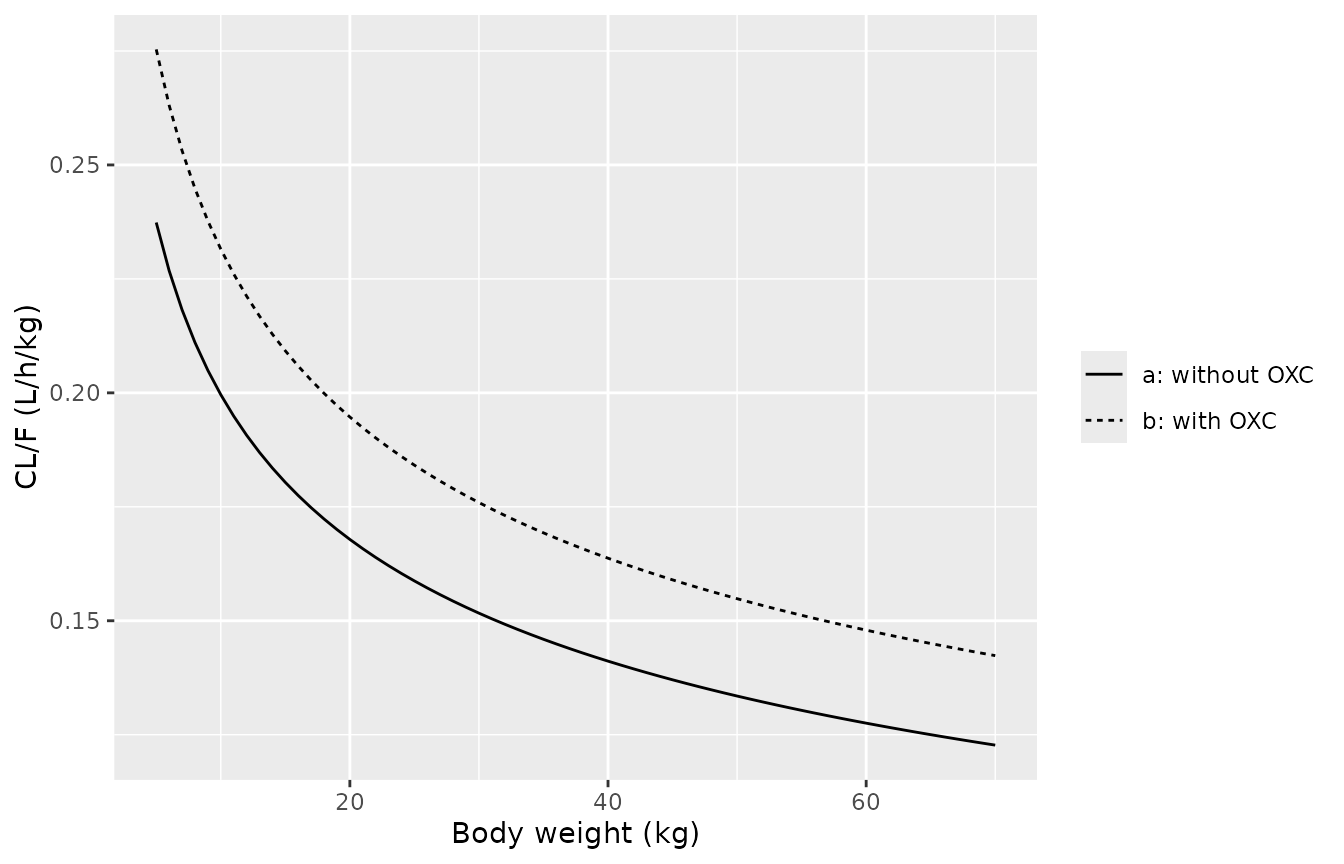
Typical sirolimus CL/F per kg body weight without (line a) and with (line b) oxcarbazepine. Replicates Figure 1E of Chen 2021.
ratio <- cl_sim |>
  select(WT, CONMED_OXC, cl) |>
  tidyr::pivot_wider(names_from = CONMED_OXC, values_from = cl, names_prefix = "oxc") |>
  mutate(ratio = oxc1 / oxc0)
# Typical values on both sides; the ratio is exact.
stopifnot(all(abs(ratio$ratio - 1.16) < 1e-8))
PKNCA validation
The paper reports no NCA. As a structural check, typical-value
children (zeroRe()) at 5, 10, 20, 40 and 70 kg, with and
without oxcarbazepine, receive 0.05 mg/kg once daily for 14 days. PKNCA
computes the steady-state AUC over the last dosing interval, which must
equal the closed form Dose / (CL/F).
nca_wt <- c(5, 10, 20, 40, 70)
tlast <- (ndays - 1) * 24
nca_grid <- tidyr::expand_grid(WT = nca_wt, CONMED_OXC = c(0, 1)) |>
  mutate(id = row_number(), treatment = sprintf("%g kg, OXC=%d", WT, CONMED_OXC))
ev_nca <- lapply(seq_len(nrow(nca_grid)), function(i) {
  g <- nca_grid[i, ]
  dose <- tibble(time = seq(0, by = 24, length.out = ndays), amt = 0.05 * g$WT, evid = 1L, cmt = "depot")
  obs <- tibble(
    time = tlast + c(0, 0.5, 1, 2, 3, 4, 5, 6, 8, 10, 12, 16, 20, 24),
    amt = 0, evid = 0L, cmt = "central"
  )
  bind_rows(dose, obs) |>
    mutate(id = g$id, WT = g$WT, CONMED_OXC = g$CONMED_OXC, treatment = g$treatment)
}) |>
  bind_rows() |>
  arrange(id, time, desc(evid))

sim_nca <- rxode2::rxSolve(mod_typ, events = ev_nca, keep = c("WT", "CONMED_OXC", "treatment")) |>
  as.data.frame()
#> ℹ omega/sigma items treated as zero: 'etalcl'
#> Warning: multi-subject simulation without without 'omega'

conc <- sim_nca |>
  filter(!is.na(Cc), time >= tlast) |>
  select(id, time, Cc, treatment)
doses <- ev_nca |>
  filter(evid == 1, time == tlast) |>
  select(id, time, amt, treatment)

o_conc <- PKNCAconc(conc, Cc ~ time | treatment + id)
o_dose <- PKNCAdose(doses, amt ~ time | treatment + id)
intervals <- data.frame(start = tlast, end = tlast + 24, auclast = TRUE, cmax = TRUE, cmin = TRUE, tmax = TRUE)
nca_res <- pk.nca(PKNCAdata(o_conc, o_dose, intervals = intervals))

nca_wide <- as.data.frame(nca_res) |>
  select(treatment, PPTESTCD, PPORRES) |>
  tidyr::pivot_wider(names_from = PPTESTCD, values_from = PPORRES) |>
  left_join(nca_grid, by = "treatment") |>
  mutate(auc_closed = 1000 * 0.05 * WT / (8.59 * (WT / 70)^0.75 * 1.16^CONMED_OXC)) |>
  arrange(CONMED_OXC, WT)

nca_wide |>
  select(treatment, auclast, auc_closed, cmax, tmax, cmin) |>
  dplyr::rename(
    "Group" = treatment, "AUCtau (PKNCA, ng*h/mL)" = auclast,
    "Dose/(CL/F) (ng*h/mL)" = auc_closed, "Cmax (ng/mL)" = cmax,
    "Tmax (h)" = tmax, "Cmin (ng/mL)" = cmin
  ) |>
knitr::kable(digits = 2, caption = "Typical-value steady-state NCA, 0.05 mg/kg once daily.")| Group | AUCtau (PKNCA, ng*h/mL) | Dose/(CL/F) (ng*h/mL) | Cmax (ng/mL) | Tmax (h) | Cmin (ng/mL) |
|---|---|---|---|---|---|
| 5 kg, OXC=0 | 210.20 | 210.64 | 12.54 | 4 | 4.68 |
| 10 kg, OXC=0 | 250.05 | 250.50 | 14.14 | 4 | 6.20 |
| 20 kg, OXC=0 | 297.45 | 297.89 | 16.08 | 5 | 8.06 |
| 40 kg, OXC=0 | 353.81 | 354.25 | 18.40 | 5 | 10.31 |
| 70 kg, OXC=0 | 406.99 | 407.45 | 20.60 | 5 | 12.46 |
| 5 kg, OXC=1 | 181.14 | 181.59 | 11.38 | 4 | 3.60 |
| 10 kg, OXC=1 | 215.50 | 215.94 | 12.75 | 4 | 4.88 |
| 20 kg, OXC=1 | 256.36 | 256.80 | 14.40 | 4 | 6.45 |
| 40 kg, OXC=1 | 304.95 | 305.39 | 16.39 | 5 | 8.36 |
| 70 kg, OXC=1 | 350.81 | 351.25 | 18.28 | 5 | 10.19 |
Assumptions and deviations
-
IIV scale. Table 2 reports “omega CL/F = 0.175”
without stating whether it is a variance or an SD. Simulating Figures
2-5 under both readings settles it: with 0.175 as the SD of eta
(variance 0.030625) the simulated probabilities reproduce the printed
percentages (e.g. 20 kg once daily at 0.04 mg/kg/day: about 80% vs 82.0%
published), whereas treating 0.175 as the variance flattens every curve
to a plateau near 40%. The SD reading is used, which is also the
convention of this group’s other pediatric TDM models
(e.g.
Wang_2019b_tacrolimus). - Residual error scale. sigma 1 = 1.913 (additive) is taken as an SD in ng/mL, consistent with the SD convention established for omega above. The paper offers no independent check; if it were a variance the SD would be 1.383 ng/mL. It does not affect the Figure 2-6 replication, which is reproduced by the individual predictions without residual error (adding an additive SD of 1.9 ng/mL lowers the 80-90% plateaus by 15-20 percentage points).
- Target attainment. The probability is read as P(5 ng/mL <= trough <= 10 ng/mL) at steady state, with the trough taken at the end of the dosing interval (24 h once daily, 12 h twice daily).
- Linear dose scaling. Each child is simulated at 0.01 mg/kg/day and the trough at higher doses is obtained by proportional scaling. This is exact for the linear model without residual error, and uses the same children across doses rather than an independent cohort per dose as in the paper.
- Oxcarbazepine indicator. The paper does not state whether the indicator was time-varying; it is accepted per record.
-
Screened covariates. Dosage form (tablet vs oral
solution) and the laboratory indices in Table 1 were screened and not
retained; dosage form is recorded under
covariatesDataExcluded. -
Fixed ka is inherited from the group’s earlier
sirolimus model (Wang
- and is not identifiable from trough-only data.
- The body-weight reference (70 kg) is near the top of the observed range (8-68 kg); the typical CL/F of 8.59 L/h is therefore an adult-equivalent value.