Unbound ceftolozane and tazobactam during CVVHDF (Sime 2019b)
Source:vignettes/articles/Sime_2019b_ceftolozane_tazobactam.Rmd
Sime_2019b_ceftolozane_tazobactam.RmdModel and source
Sime et al. fitted the two analytes of the fixed 2:1
ceftolozane-tazobactam combination as two separate nonparametric
(Pmetrics NPAG) models sharing one four-compartment structure, so the
paper contributes two model files. The b
in the file names distinguishes this paper from the same group’s 2019
study of the same drug in patients without renal dysfunction
(Sime_2019_ceftolozane / Sime_2019_tazobactam,
doi:10.1128/AAC.01265-19).
cef <- rxode2::rxode(readModelDb("Sime_2019b_ceftolozane"))
#> ℹ parameter labels from comments will be replaced by 'label()'
taz <- rxode2::rxode(readModelDb("Sime_2019b_tazobactam"))
#> ℹ parameter labels from comments will be replaced by 'label()'- Citation: Sime FB, Lassig-Smith M, Starr T, Stuart J, Pandey S, Parker SL, Wallis SC, Lipman J, Roberts JA. A population pharmacokinetic model-guided evaluation of ceftolozane-tazobactam dosing in critically ill patients undergoing continuous venovenous hemodiafiltration. Antimicrob Agents Chemother. 2019 (published 20 December 2019; issue January 2020);64(1):e01655-19. doi:10.1128/AAC.01655-19. PMCID: PMC7187594. Structure: Figure 1. All parameter values: Table 3, ‘Ceftolozane’ columns.
- Article: https://doi.org/10.1128/AAC.01655-19 (PMCID: PMC7187594, open access)
- Ceftolozane: Four-compartment intravenous population PK model for UNBOUND ceftolozane in six critically ill adults undergoing continuous venovenous hemodiafiltration (CVVHDF) in a quaternary referral intensive care unit in Brisbane, Australia. Fitted non-parametrically in Pmetrics (NPAG) to unbound prefilter plasma, postfilter plasma and CVVHDF effluent concentrations simultaneously. A prefilter central compartment receives the dose and loses drug by residual non-CVVHDF clearance and by CVVHDF clearance into an effluent compartment, which drains first-order; it exchanges with a postfilter compartment by the rate constants K12 / K21 and with a peripheral compartment by an intercompartmental clearance, and the postfilter compartment also exchanges with the same peripheral compartment (paper Figure 1). No covariate was retained. Every parameter carries its own inter-individual variability taken from the mean and SD of the NPAG support-point distribution; residual error is fixed(0) because the selected Pmetrics error model was not published. Ceftolozane and tazobactam were fitted as separate models and are supplied as two files; see modellib(‘Sime_2019b_tazobactam’) for the partner component of the fixed 2:1 ceftolozane-tazobactam combination.
- Tazobactam: Four-compartment intravenous population PK model for UNBOUND tazobactam in six critically ill adults undergoing continuous venovenous hemodiafiltration (CVVHDF) in a quaternary referral intensive care unit in Brisbane, Australia. Fitted non-parametrically in Pmetrics (NPAG) to unbound prefilter plasma, postfilter plasma and CVVHDF effluent concentrations simultaneously. A prefilter central compartment receives the dose and loses drug by residual non-CVVHDF clearance and by CVVHDF clearance into an effluent compartment, which drains first-order; it exchanges with a postfilter compartment by the rate constants K12 / K21 and with a peripheral compartment by an intercompartmental clearance, and the postfilter compartment also exchanges with the same peripheral compartment (paper Figure 1). No covariate was retained. Every parameter carries its own inter-individual variability taken from the mean and SD of the NPAG support-point distribution; residual error is fixed(0) because the selected Pmetrics error model was not published. Ceftolozane and tazobactam were fitted as separate models and are supplied as two files; see modellib(‘Sime_2019b_ceftolozane’) for the partner component of the fixed 2:1 ceftolozane-tazobactam combination.
The structure is the paper’s Figure 1. The dose is infused into the
prefilter compartment (central, volume V_pre), which loses
drug by a residual non-CVVHDF clearance (cl) and by the
CVVHDF clearance (cl_crrt) into an effluent compartment
(circuit_dialysate, volume V_effluent) that drains at the
first-order rate Kd. The prefilter compartment also exchanges with a
postfilter compartment (postfilter, V_post) through the
rate constants K12 / K21 and with a peripheral compartment
(peripheral1, V_peripheral) through Q_pre; the postfilter
compartment exchanges with the same peripheral compartment through
Q_post. The three fitted outputs are the unbound prefilter plasma
concentration Cc, the unbound postfilter plasma
concentration Cpostfilter, and the effluent concentration
Ceffluent.
All concentrations are UNBOUND. The assay isolated the unbound fraction by ultracentrifugation before measurement, so no protein-binding conversion appears in either file.
Population
Six critically ill adults in the intensive care unit of the Royal Brisbane and Women’s Hospital, Australia, all on continuous venovenous hemodiafiltration (CVVHDF) with a Prismaflex machine and an AN69 ST100 or ST150 filter (Tables 1 and 2). Five were male. Median age was 61.5 years (Q1-Q3 58-65; range 23-66), median weight 72.5 kg (65-95), median serum creatinine 138 umol/L, median albumin 26.5 g/L, median APACHE II 32 and median SOFA 11.5. Blood flow rates were 100-200 mL/min and dialysate flow rates 1,000-1,500 mL/h. Every patient received 1.5 g ceftolozane-tazobactam (1000 mg ceftolozane + 500 mg tazobactam) every 8 h as a 1-h infusion, and was sampled over one dosing interval in prefilter plasma, postfilter plasma and effluent.
Source trace
| Quantity | Ceftolozane | Tazobactam | Source |
|---|---|---|---|
| Structure (4 compartments, clearances, transfers) | – | – | Figure 1 and its legend |
CL_CVVHDF (L/h), lcl_crrt
|
2.659 (SD 0.783) | 2.973 (SD 0.603) | Table 3 |
CL_residual (L/h), lcl
|
0.596 (SD 0.504) | 3.254 (SD 0.867) | Table 3 |
V_pre (L), lvc
|
25.184 (SD 7.499) | 28.206 (SD 6.603) | Table 3 |
V_post (L), lvpostfilter
|
17.578 (SD 10.871) | 19.685 (SD 14.382) | Table 3 |
K12 (1/h), lk12
|
0.43 (SD 0.718) | 0.561 (SD 0.638) | Table 3 |
K21 (1/h), lk21
|
0.676 (SD 0.908) | 1.01 (SD 1.01) | Table 3 |
Kd (1/h), lkd
|
1.596 (SD 0.495) | 1.584 (SD 0.483) | Table 3 |
V_effluent (L), lvdialysate
|
2.178 (SD 0.801) | 2.609 (SD 1.561) | Table 3 |
Q_pre (L/h), lq
|
0.834 (SD 1.863) | 2.547 (SD 2.455) | Table 3 |
Q_post (L/h), lqpostfilter
|
2.42 (SD 1.451) | 3.612 (SD 1.204) | Table 3 |
V_peripheral (L), lvp
|
73.379 (SD 39.042) | 77.196 (SD 32.267) | Table 3 |
IIV, eta*
|
log((SD/mean)^2 + 1) | same | Table 3 SD column |
| Residual error | fixed(0) | fixed(0) | not reported (Methods) |
| Dose split 2:1 | 1000 mg per 1.5 g | 500 mg per 1.5 g | Methods, ‘Ceftolozane-tazobactam dosing’ |
The IIV variances are derived from the transcribed values. This check is pure arithmetic on the model files, so it is asserted tightly.
tab3 <- data.frame(
  eta = c(
    "etalcl_crrt", "etalcl", "etalvc", "etalvpostfilter", "etalk12", "etalk21",
    "etalkd", "etalvdialysate", "etalq", "etalqpostfilter", "etalvp"
  ),
  cef_mean = c(2.659, 0.596, 25.184, 17.578, 0.43, 0.676, 1.596, 2.178, 0.834, 2.42, 73.379),
  cef_sd = c(0.783, 0.504, 7.499, 10.871, 0.718, 0.908, 0.495, 0.801, 1.863, 1.451, 39.042),
  taz_mean = c(2.973, 3.254, 28.206, 19.685, 0.561, 1.01, 1.584, 2.609, 2.547, 3.612, 77.196),
  taz_sd = c(0.603, 0.867, 6.603, 14.382, 0.638, 1.01, 0.483, 1.561, 2.455, 1.204, 32.267)
)
om_cef <- diag(cef$omega)[tab3$eta]
om_taz <- diag(taz$omega)[tab3$eta]
stopifnot(
  all(abs(om_cef - log((tab3$cef_sd / tab3$cef_mean)^2 + 1)) < 1e-4),
  all(abs(om_taz - log((tab3$taz_sd / tab3$taz_mean)^2 + 1)) < 1e-4)
)
tab3 |>
  mutate(cef_cv = round(100 * cef_sd / cef_mean), taz_cv = round(100 * taz_sd / taz_mean)) |>
  select(eta, cef_cv, taz_cv) |>
  rename("Random effect" = eta, "Ceftolozane CV (%)" = cef_cv, "Tazobactam CV (%)" = taz_cv) |>
knitr::kable()| Random effect | Ceftolozane CV (%) | Tazobactam CV (%) |
|---|---|---|
| etalcl_crrt | 29 | 20 |
| etalcl | 85 | 27 |
| etalvc | 30 | 23 |
| etalvpostfilter | 62 | 73 |
| etalk12 | 167 | 114 |
| etalk21 | 134 | 100 |
| etalkd | 31 | 30 |
| etalvdialysate | 37 | 60 |
| etalq | 223 | 96 |
| etalqpostfilter | 60 | 33 |
| etalvp | 53 | 42 |
Virtual cohorts
The paper’s simulations drew 1,000 virtual patients from the NPAG support points. Here each regimen gets 150 virtual patients drawn from the independent log-normal marginals encoded in the model files. There are no covariates to sample. The regimens are a subset of Tables 4, 5 and S1; the combination dose is split 2:1 between the two analytes.
n_per_arm <- 150
regimens <- tibble::tribble(
  ~regimen, ~combo_g, ~type, ~dur,
  "0.375 g q8h", 0.375, "intermittent", 1,
  "0.75 g q8h", 0.75, "intermittent", 1,
  "1.5 g q8h", 1.5, "intermittent", 1,
  "3.0 g q8h", 3.0, "intermittent", 1,
  "1.5 g 4 h EI q8h", 1.5, "intermittent", 4,
  "1.5 g LD + 4.5 g CI", 1.5, "continuous", 1
)
n_days <- 10
tau <- 8

# Dose rows for one regimen, in mg of one analyte. The continuous-infusion
# arm is a 1-h loading dose followed, from the end of the loading dose, by the
# daily dose (3 x the q8h dose) infused over each 24 h.
dose_rows <- function(reg, frac, ids) {
  amt1 <- reg$combo_g * 1000 * frac
  if (reg$type == "intermittent") {
    t_dose <- seq(0, n_days * 24 - tau, by = tau)
    d <- expand.grid(id = ids, time = t_dose)
    d$amt <- amt1
    d$rate <- amt1 / reg$dur
  } else {
    ld <- data.frame(id = ids, time = 0, amt = amt1, rate = amt1)
    t_ci <- 1 + seq(0, (n_days - 1) * 24, by = 24)
    ci <- expand.grid(id = ids, time = t_ci)
    ci$amt <- 3 * amt1
    ci$rate <- 3 * amt1 / 24
    d <- rbind(ld, ci)
  }
  d$evid <- 1L
  d$cmt <- "central"
  d$dvid <- NA_integer_
  d
}

obs_times <- sort(unique(c(seq(0, 24, by = 0.1), 96, seq(216, 224, by = 0.1))))

build_events <- function(frac) {
  out <- lapply(seq_len(nrow(regimens)), function(i) {
    ids <- (i - 1) * n_per_arm + seq_len(n_per_arm)
    obs <- expand.grid(id = ids, time = obs_times)
    obs$amt <- NA_real_
    obs$rate <- NA_real_
    obs$evid <- 0L
    # Three endpoints are declared, so observation rows are keyed by dvid
    # with no cmt; every output (Cc, Cpostfilter, Ceffluent) is returned on
    # each row.
    obs$cmt <- NA_character_
    obs$dvid <- 1L
    ev <- rbind(dose_rows(regimens[i, ], frac, ids), obs)
    ev$regimen <- regimens$regimen[i]
    ev
  })
  ev <- do.call(rbind, out)
  ev[order(ev$id, ev$time, -ev$evid), ]
}
ev_cef <- build_events(2 / 3)
ev_taz <- build_events(1 / 3)
Simulation
# rxSetSeed() fixes the draw within one rxode2 build and thread count only;
# every assertion below is written on medians and robust proportions so that
# it holds for any cohort the model can produce.
rxode2::rxSetSeed(20191220)
# sigma = NA: residual error is fixed(0) and is not simulated.
sim_cef <- rxode2::rxSolve(cef, ev_cef, sigma = NA, keep = "regimen", returnType = "data.frame")
sim_taz <- rxode2::rxSolve(taz, ev_taz, sigma = NA, keep = "regimen", returnType = "data.frame")
sim <- bind_rows(
  mutate(sim_cef, drug = "ceftolozane"),
  mutate(sim_taz, drug = "tazobactam")
)
# Solver sanity: all four states survive and nothing goes negative.
stopifnot(
  all(sim$Cc >= -1e-8), all(sim$Cpostfilter >= -1e-8), all(sim$Ceffluent >= -1e-8),
  max(sim$peripheral1) > 0, max(sim$postfilter) > 0
)
Typical-value profiles in the three fitted matrices
Replicates the matrices of Figures 2 and 3 (prefilter, postfilter and effluent) as typical-value curves over the first 24 h of 1.5 g q8h. The paper’s own figures are observed-versus-predicted scatter plots, which need the individual data.
typ_events <- function(frac) {
  d <- dose_rows(regimens[regimens$regimen == "1.5 g q8h", ], frac, 1L)
  o <- data.frame(
    id = 1L, time = obs_times, amt = NA_real_, rate = NA_real_, evid = 0L,
    cmt = NA_character_, dvid = 1L
  )
  r <- rbind(d, o)
  r[order(r$time, -r$evid), ]
}
typ <- bind_rows(
  mutate(rxode2::rxSolve(cef, typ_events(2 / 3), omega = NA, sigma = NA, returnType = "data.frame"), drug = "ceftolozane"),
  mutate(rxode2::rxSolve(taz, typ_events(1 / 3), omega = NA, sigma = NA, returnType = "data.frame"), drug = "tazobactam")
)
typ |>
  filter(time <= 24) |>
  select(time, drug, Prefilter = Cc, Postfilter = Cpostfilter, Effluent = Ceffluent) |>
  pivot_longer(c(Prefilter, Postfilter, Effluent), names_to = "matrix", values_to = "conc") |>
  ggplot(aes(time, conc, colour = matrix)) +
  geom_line() +
  facet_wrap(~drug, scales = "free_y") +
  labs(x = "Time (h)", y = "Unbound concentration (mg/L)", colour = NULL) +
  theme_bw()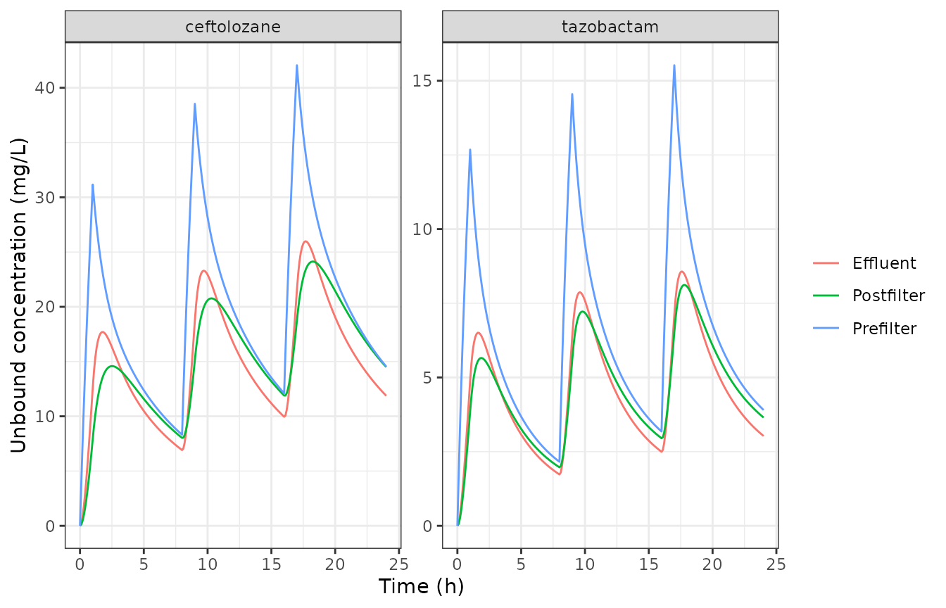
Prefilter percentiles over the first dosing interval
Supplemental Figure S1 is a visual predictive check of prefilter plasma during the sampled dosing interval. The sampled interval’s position in each patient’s course is not stated, so the check is not replicated quantitatively; the first-interval percentiles below show the same 5th-95th percentile layout.
sim |>
  filter(regimen == "1.5 g q8h", time <= 8) |>
  group_by(drug, time) |>
  summarise(
    p05 = quantile(Cc, 0.05), p25 = quantile(Cc, 0.25), p50 = median(Cc),
    p75 = quantile(Cc, 0.75), p95 = quantile(Cc, 0.95), .groups = "drop"
  ) |>
  ggplot(aes(time)) +
  geom_ribbon(aes(ymin = p05, ymax = p95), fill = "grey85") +
  geom_ribbon(aes(ymin = p25, ymax = p75), fill = "grey65") +
  geom_line(aes(y = p50)) +
  facet_wrap(~drug, scales = "free_y") +
  labs(x = "Time after first dose (h)", y = "Unbound prefilter concentration (mg/L)") +
  theme_bw()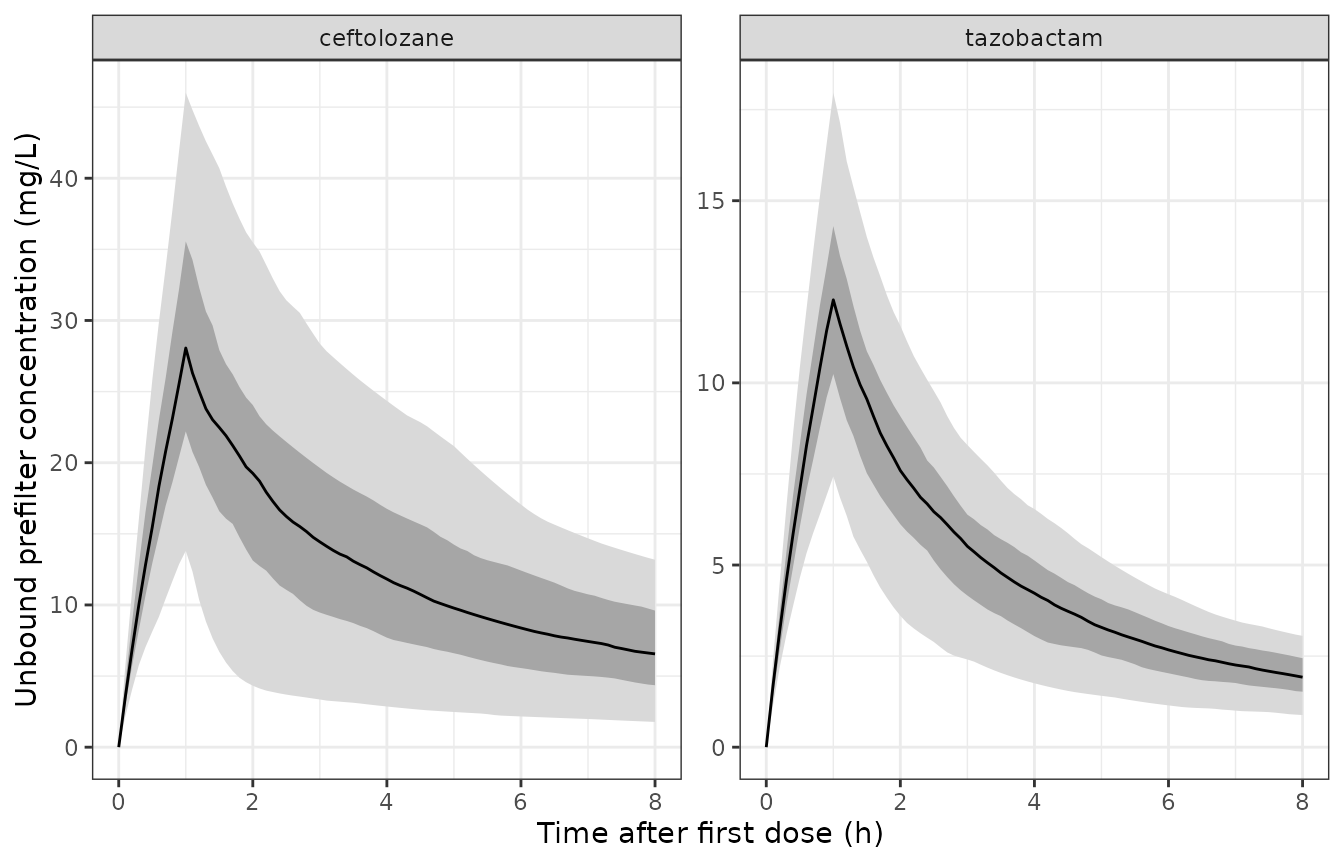
PKNCA validation
Steady-state NCA over the last dosing interval (216-224 h) of every regimen, for each analyte, compared against the medians of Table 5. For intermittent regimens Cmax is the end-of-infusion concentration of Table 5 and Cmin its trough; for the continuous infusion Table 5 reports only the steady-state concentration, compared against Cmin.
run_nca <- function(s, ev) {
  conc <- s |>
    filter(!is.na(Cc)) |>
    select(id, time, Cc, regimen)
  dose <- ev |>
    filter(evid == 1) |>
    select(id, time, amt, regimen)
  conc_obj <- PKNCA::PKNCAconc(conc, Cc ~ time | regimen + id, concu = "mg/L", timeu = "h")
  dose_obj <- PKNCA::PKNCAdose(dose, amt ~ time | regimen + id, doseu = "mg")
  intervals <- data.frame(start = 216, end = 224, cmax = TRUE, cmin = TRUE, auclast = TRUE)
  PKNCA::pk.nca(PKNCA::PKNCAdata(conc_obj, dose_obj, intervals = intervals))
}
nca_cef <- run_nca(sim_cef, ev_cef)
nca_taz <- run_nca(sim_taz, ev_taz)

# Table 5, median steady-state concentrations (mg/L).
ref_cef <- data.frame(
  regimen = regimens$regimen,
  cmax = c(13, 27, 54, 107, 44, NA),
  cmin = c(7, 14, 28, 56, 31, 36)
)
ref_taz <- data.frame(
  regimen = regimens$regimen,
  cmax = c(4.4, 8.8, 17.5, 35.0, 12.3, NA),
  cmin = c(1.5, 3.0, 6.1, 12.1, 7.0, 9.7)
)
cmp_cef <- ncaComparisonTable(nca_cef, ref_cef, by = "regimen", params = c("cmax", "cmin"), units = c(cmax = "mg/L", cmin = "mg/L"))
cmp_taz <- ncaComparisonTable(nca_taz, ref_taz, by = "regimen", params = c("cmax", "cmin"), units = c(cmax = "mg/L", cmin = "mg/L"))
knitr::kable(cmp_cef, caption = "Ceftolozane, steady state: simulated median vs Table 5 median.")| NCA parameter | regimen | Reference | Simulated | % diff |
|---|---|---|---|---|
| Cmax (mg/L) | 0.375 g q8h | 13 | 13.4 | +3.4% |
| Cmax (mg/L) | 0.75 g q8h | 27 | 27.1 | +0.3% |
| Cmax (mg/L) | 1.5 g q8h | 54 | 54 | +0.1% |
| Cmax (mg/L) | 3.0 g q8h | 107 | 109 | +2.2% |
| Cmax (mg/L) | 1.5 g 4 h EI q8h | 44 | 40 | -9.1% |
| Cmax (mg/L) | 1.5 g LD + 4.5 g CI | — | 35.1 | — |
| Cmin (mg/L) | 0.375 g q8h | 7 | 6.42 | -8.3% |
| Cmin (mg/L) | 0.75 g q8h | 14 | 12 | -14.2% |
| Cmin (mg/L) | 1.5 g q8h | 28 | 25.4 | -9.1% |
| Cmin (mg/L) | 3.0 g q8h | 56 | 49.1 | -12.3% |
| Cmin (mg/L) | 1.5 g 4 h EI q8h | 31 | 26.1 | -15.9% |
| Cmin (mg/L) | 1.5 g LD + 4.5 g CI | 36 | 35.1 | -2.4% |
knitr::kable(cmp_taz, caption = "Tazobactam, steady state: simulated median vs Table 5 median.")| NCA parameter | regimen | Reference | Simulated | % diff |
|---|---|---|---|---|
| Cmax (mg/L) | 0.375 g q8h | 4.4 | 4.43 | +0.6% |
| Cmax (mg/L) | 0.75 g q8h | 8.8 | 9.13 | +3.7% |
| Cmax (mg/L) | 1.5 g q8h | 17.5 | 18 | +2.7% |
| Cmax (mg/L) | 3.0 g q8h | 35 | 36.5 | +4.3% |
| Cmax (mg/L) | 1.5 g 4 h EI q8h | 12.3 | 12.4 | +0.7% |
| Cmax (mg/L) | 1.5 g LD + 4.5 g CI | — | 9.88 | — |
| Cmin (mg/L) | 0.375 g q8h | 1.5 | 1.58 | +5.0% |
| Cmin (mg/L) | 0.75 g q8h | 3 | 3.16 | +5.4% |
| Cmin (mg/L) | 1.5 g q8h | 6.1 | 6.1 | -0.0% |
| Cmin (mg/L) | 3.0 g q8h | 12.1 | 12.1 | -0.2% |
| Cmin (mg/L) | 1.5 g 4 h EI q8h | 7 | 6.91 | -1.3% |
| Cmin (mg/L) | 1.5 g LD + 4.5 g CI | 9.7 | 9.86 | +1.6% |
# Recompute the percentage differences numerically for the gate.
pct <- function(nca, ref) {
  as.data.frame(nca$result) |>
    filter(PPTESTCD %in% c("cmax", "cmin")) |>
    group_by(regimen, PPTESTCD) |>
    summarise(sim = median(PPORRES), .groups = "drop") |>
    inner_join(pivot_longer(ref, c(cmax, cmin), names_to = "PPTESTCD", values_to = "ref"), by = c("regimen", "PPTESTCD")) |>
    filter(!is.na(ref)) |>
    mutate(pct_diff = 100 * (sim - ref) / ref)
}
chk <- bind_rows(pct(nca_cef, ref_cef), pct(nca_taz, ref_taz))
stopifnot(
  # Structural: a wrong clearance, dose split or unit moves every row by tens
  # of percent.
  abs(median(chk$pct_diff)) < 10,
  # Envelope on per-regimen MEDIANS (not extremes); Table 5 rounds the small
  # tazobactam values to one or two significant figures.
  quantile(abs(chk$pct_diff), 0.9) < 25
)
Closed-form checks
The system is linear, so for the typical patient the steady-state AUC over one interval must equal dose / (CL_residual + CL_CVVHDF), and the drug removed into the effluent over that interval must be the fraction CL_CVVHDF / (CL_residual + CL_CVVHDF) of the dose. Both are deterministic (no cohort draw), so the bounds are tight.
# The slowly equilibrating peripheral compartment leaves the typical patient
# about 0.7% short of true steady state at day 10, so the identity is checked
# on the last interval of a 40-day regimen on a 0.02 h grid.
long_typ <- function(mod, amt) {
  d <- data.frame(
    id = 1L, time = seq(0, 40 * 24 - tau, by = tau), amt = amt, rate = amt,
    evid = 1L, cmt = "central", dvid = NA_integer_
  )
  o <- data.frame(
    id = 1L, time = seq(40 * 24 - tau, 40 * 24, by = 0.02), amt = NA_real_,
    rate = NA_real_, evid = 0L, cmt = NA_character_, dvid = 1L
  )
  e <- rbind(d, o)
  rxode2::rxSolve(mod, e[order(e$time, -e$evid), ], omega = NA, sigma = NA, returnType = "data.frame")
}
cf <- bind_rows(
  mutate(long_typ(cef, 1000), drug = "ceftolozane"),
  mutate(long_typ(taz, 500), drug = "tazobactam")
) |>
  group_by(drug) |>
  summarise(
    auc = sum(diff(time) * (head(Cc, -1) + tail(Cc, -1)) / 2),
    .groups = "drop"
  ) |>
  mutate(
    dose = c(1000, 500),
    cl_tot = c(0.596 + 2.659, 3.254 + 2.973),
    auc_expected = dose / cl_tot,
    pct_diff = 100 * (auc - auc_expected) / auc_expected,
    frac_cvvhdf = c(2.659, 2.973) / cl_tot
  )
knitr::kable(cf, digits = 3)| drug | auc | dose | cl_tot | auc_expected | pct_diff | frac_cvvhdf |
|---|---|---|---|---|---|---|
| ceftolozane | 307.220 | 1000 | 3.255 | 307.220 | 0 | 0.817 |
| tazobactam | 80.295 | 500 | 6.227 | 80.295 | 0 | 0.477 |
The paper gives total ceftolozane clearance during CVVHDF as 3.3 L/h
(Discussion), i.e. 0.596 + 2.659 = 3.255 L/h. From Table 3, about 82% of
ceftolozane clearance but only 48% of tazobactam clearance is
extracorporeal (the frac_cvvhdf column).
The Discussion also states that “steady state was achieved only after 4 days for ceftolozane”. Below, the typical-patient pre-dose trough on each of days 1-6 of 1.5 g q8h is expressed as a fraction of the day-40 trough (true steady state). Doubling the dose must double the concentration exactly (Results, “doubling the dose resulted in doubling the steady-state concentration”).
daily_trough <- function(mod, amt) {
  d <- data.frame(
    id = 1L, time = seq(0, 40 * 24 - tau, by = tau), amt = amt, rate = amt,
    evid = 1L, cmt = "central", dvid = NA_integer_
  )
  o <- data.frame(
    id = 1L, time = seq(24, 40 * 24, by = 24), amt = NA_real_,
    rate = NA_real_, evid = 0L, cmt = NA_character_, dvid = 1L
  )
  e <- rbind(d, o)
  s <- rxode2::rxSolve(mod, e[order(e$time, -e$evid), ], omega = NA, sigma = NA, returnType = "data.frame")
  s$Cc / s$Cc[s$time == 40 * 24]
}
ss_frac <- data.frame(
  day = 1:6,
  ceftolozane = daily_trough(cef, 1000)[1:6],
  tazobactam = daily_trough(taz, 500)[1:6]
)
knitr::kable(ss_frac, digits = 3, caption = "Typical pre-dose trough as a fraction of the steady-state trough.")| day | ceftolozane | tazobactam |
|---|---|---|
| 1 | 0.518 | 0.634 |
| 2 | 0.692 | 0.840 |
| 3 | 0.801 | 0.930 |
| 4 | 0.872 | 0.969 |
| 5 | 0.918 | 0.987 |
| 6 | 0.947 | 0.994 |
# Deterministic (typical values, no cohort draw). Ceftolozane is well short of
# steady state at day 2 and within ~15% of it by day 4; tazobactam, with twice
# the clearance, gets there sooner.
stopifnot(
  ss_frac$ceftolozane[2] < 0.8,
  ss_frac$ceftolozane[4] > 0.85,
  all(ss_frac$tazobactam > ss_frac$ceftolozane)
)

trough <- function(d, t) d$Cc[which.min(abs(d$time - t))]
typ_double <- rxode2::rxSolve(cef, transform(typ_events(2 / 3), amt = 2 * amt, rate = 2 * rate), omega = NA, sigma = NA, returnType = "data.frame")
stopifnot(abs(trough(typ_double, 224) / trough(filter(typ, drug == "ceftolozane"), 224) - 2) < 1e-6)
Probability of target attainment
%fT above a threshold is computed from the prefilter concentration (Methods: “Prefilter patient plasma exposure was used for all PTA assessments”) over the first 24 h and over the steady-state interval 216-224 h.
ft_above <- function(d, thr, t0, t1) {
  x <- d[d$time >= t0 & d$time <= t1, ]
  mean(x$Cc > thr)
}
pta <- function(drug_name, thr, target_pct, t0, t1) {
  sim |>
    filter(drug == drug_name) |>
    group_by(regimen, id) |>
    group_modify(~ data.frame(ft = ft_above(.x, thr, t0, t1))) |>
    group_by(regimen) |>
    summarise(pta = mean(100 * ft >= target_pct), .groups = "drop")
}
pta_tab <- bind_rows(
  mutate(pta("ceftolozane", 4, 40, 0, 24), target = "Ceftolozane 40% fT>4 mg/L, first 24 h"),
  mutate(pta("tazobactam", 1, 20, 0, 24), target = "Tazobactam 20% fT>1 mg/L, first 24 h"),
  mutate(pta("tazobactam", 2, 50, 0, 24), target = "Tazobactam 50% fT>2 mg/L, first 24 h"),
  mutate(pta("tazobactam", 4, 100, 216, 224), target = "Tazobactam 100% fT>4 mg/L, steady state")
)
pta_tab |>
  pivot_wider(names_from = regimen, values_from = pta) |>
knitr::kable(digits = 2)| target | 0.375 g q8h | 0.75 g q8h | 1.5 g 4 h EI q8h | 1.5 g LD + 4.5 g CI | 1.5 g q8h | 3.0 g q8h |
|---|---|---|---|---|---|---|
| Ceftolozane 40% fT>4 mg/L, first 24 h | 0.63 | 0.88 | 1.00 | 1.00 | 0.97 | 1.00 |
| Tazobactam 20% fT>1 mg/L, first 24 h | 0.95 | 1.00 | 1.00 | 1.00 | 1.00 | 1.00 |
| Tazobactam 50% fT>2 mg/L, first 24 h | 0.03 | 0.83 | 0.97 | 0.99 | 0.98 | 0.99 |
| Tazobactam 100% fT>4 mg/L, steady state | 0.00 | 0.18 | 0.98 | 1.00 | 0.88 | 1.00 |
get_pta <- function(tgt, reg) pta_tab$pta[pta_tab$target == tgt & pta_tab$regimen == reg]
stopifnot(
  # Results: PTA >= 0.9 for 40% fT>MIC at MIC 4 mg/L in the first 24 h. The
  # floor sits below 0.9 to absorb the cohort draw; 0.375 g q8h is excluded
  # (see the deviation noted below the table).
  all(sapply(setdiff(regimens$regimen, "0.375 g q8h"), function(r) get_pta("Ceftolozane 40% fT>4 mg/L, first 24 h", r)) > 0.8),
  # Table S1: 20% fT>1 mg/L was 1.0 for every regimen.
  all(sapply(regimens$regimen, function(r) get_pta("Tazobactam 20% fT>1 mg/L, first 24 h", r)) > 0.9),
  # Table S1: 50% fT>2 mg/L in the first 24 h 0.1 at 0.375 g q8h, 1.0 at
  # 0.75 g q8h and above.
  get_pta("Tazobactam 50% fT>2 mg/L, first 24 h", "0.375 g q8h") < 0.5,
  get_pta("Tazobactam 50% fT>2 mg/L, first 24 h", "1.5 g q8h") > 0.9,
  # Table S1: 100% fT>4 mg/L at steady state 0.0 at 0.75 g q8h, 1.0 at 1.5 g q8h.
  get_pta("Tazobactam 100% fT>4 mg/L, steady state", "0.75 g q8h") < 0.4,
  get_pta("Tazobactam 100% fT>4 mg/L, steady state", "1.5 g q8h") > 0.6
)
Two published statements are not reproduced:
- 0.375 g q8h, ceftolozane 40% fT>MIC. The Results state that all simulated regimens reached PTA >= 0.9 for 40% fT>MIC at MIC <= 4 mg/L in the first 24 h; here 0.375 g q8h falls short (see the table). The lowest dose is also the one with the lowest cumulative fractional response in Table 4 (0.82), and the gap is consistent with the log-normal approximation to the NPAG distribution (see Assumptions and deviations).
- 100% fT above a threshold in the first 24 h (Table 4 for ceftolozane, Table S1 for tazobactam) is not computed. Over a window that starts at the first dose the concentration begins at zero, so 100% cannot be reached as defined here; the paper does not state the time grid over which its first-24 h percentages were evaluated.
Assumptions and deviations
-
Nonparametric to parametric. Table 3 summarises
each NPAG marginal as a mean and SD. Each mean is encoded as the median
of a log-normal distribution with CV = SD / mean, following the group’s
sibling models (
Sime_2019_ceftolozane,Sime_2019_tazobactam) and other Pmetrics models in the library. Several CVs exceed 100% (ceftolozane K12 167%, K21 134%, Q_pre 223%; tazobactam K12 114%, K21 100%), so the simulated population means of those parameters exceed the tabulated means. The simulated per-regimen medians nonetheless reproduce Table 5, and exposure (AUC, average concentration) depends only on the two clearances, whose CVs are 20-85%. - Parameter correlations are not recoverable from the publication, so all random effects are independent. The simulated interquartile ranges are narrower than those of Table 5 (e.g. ceftolozane 1.5 g q8h trough Q3 42 mg/L in the paper), which a discrete, correlated NPAG distribution can produce and an independent log-normal approximation does not.
-
Residual error is not reported: the Methods list
the Pmetrics error models tested but neither the selected form nor its
coefficients. All six residual parameters are
fixed(0). -
Effluent compartment name. The effluent compartment
gains drug by the CVVHDF clearance and drains first-order, which is the
role of the library’s
circuit_dialysatestate; its fitted volume (about 2 L) is an empirical quantity, not the physical dialysate-side volume of the filter. The postfilter compartment is likewise an empirical compartment and is carried under the paper-specific namepostfilter. - CVVHDF settings are fixed into the parameters. No CVVHDF setting was retained as a covariate, so the model applies only to settings similar to Table 2 (blood flow 100-200 mL/min, dialysate 1,000-1,500 mL/h).
- Continuous-infusion timing. The continuous infusion is assumed to start at the end of the 1-h loading dose.
- Supplemental Figure S1 (prefilter VPC) is shown only in layout, because the position of the sampled dosing interval in each patient’s course is not stated.