Bintrafusp alfa PK, tumour growth and multistate dose-response in NSCLC (Liu 2023)
Source:vignettes/articles/Liu_2023_bintrafuspAlfa.Rmd
Liu_2023_bintrafuspAlfa.RmdModel and source
Liu et al. (2023) analysed the second-line non-small cell lung cancer (2L NSCLC) expansion cohort of the phase I trial of bintrafusp alfa (NCT02517398), a bifunctional fusion protein that blocks PD-L1 and traps TGF-beta. Eighty patients were randomized 1:1 to 500 or 1200 mg every 2 weeks (q2w). The paper builds three models, all shipped here:
-
Liu_2023_bintrafuspAlfa– two-compartment population PK model (Appendix S1, Supplementary Table S2). -
Liu_2023_bintrafuspAlfa_tgi– tumour growth inhibition (TGI) model of the sum of longest diameters (SLD) of target lesions (Appendix S1, Supplementary Table S2). -
Liu_2023_bintrafuspAlfa_multistateandLiu_2023_bintrafuspAlfa_multistate_dose– the six-state multistate model of tumour response, progression and survival, in its final (dose-independent) form and in the dose-dependent form the authors used for their dose-response simulations (Table 2).
Neither the PK model nor the TGI model feeds the multistate model: individual clearance, dose and tumour-dynamic metrics were screened as predictors of the transitions but none was retained.
- Citation: Liu H, Milenkovic-Grisic AM, Krishnan SM, Jonsson S, Friberg LE, Girard P, Venkatakrishnan K, Vugmeyster Y, Khandelwal A, Karlsson MO. A multistate modeling and simulation framework to learn dose-response of oncology drugs: Application to bintrafusp alfa in non-small cell lung cancer. CPT Pharmacometrics Syst Pharmacol. 2023;12(11):1738-1750. doi:10.1002/psp4.12976. PMCID: PMC10681430. Equations 1-10 and Table 2 (‘Final multistate model’ column) of the main text; covariate coding from Supplementary Table S3; Gompertz-Makeham constants and the hazard code from the example NONMEM control stream in Appendix S2. Gompertz-Makeham form: Missov TI, Lenart A. Theor Popul Biol. 2013;90:29-35.
- Article (open access): https://doi.org/10.1002/psp4.12976
- PMC record with Appendices S1-S2, Supplementary Figures S1-S6 and Tables S1-S5: https://www.ncbi.nlm.nih.gov/pmc/articles/PMC10681430/
Population
The 80 patients (40 per arm) had advanced NSCLC after failure of first-line therapy; mean age 63.9 and 62.1 years (range 38-85), mean body weight 68.0 and 70.8 kg, 29% women overall (40% vs 18% by arm), 49% White and 50% Asian (Asian patients came from Korean and Taiwanese sites), all ECOG 0-1, 81% with metastases at baseline (Liu 2023 Table 1). Tumour assessments per RECIST 1.1 by independent review were scheduled every 6 weeks in the first year and every 12 weeks thereafter. The multistate data held 406 observations (75 SD, 127 PR, 124 PD and 80 absorbing events: 56 deaths, 13 dropouts, 11 censored at data cutoff).
The same information is available programmatically through each
model’s population metadata, e.g.
readModelDb("Liu_2023_bintrafuspAlfa_multistate")()$population.
Source trace
Every ini() value carries an in-file comment naming its
source. The table collects them.
| Model / parameter | Value | Source |
|---|---|---|
PK lcl
|
0.0143 L/h | Supplementary Table S2 |
PK lvc
|
3.02 L | Supplementary Table S2 |
PK lvp (fixed) |
0.483 L | Supplementary Table S2 (fixed to Wilkins 2019) |
PK lq (fixed) |
0.00512 L/h | Supplementary Table S2 (fixed to Wilkins 2019) |
PK etalcl, cov, etalvc
|
0.0795, 0.0472, 0.0424 | Supplementary Table S2 |
PK etaRUV
|
0.260 | Supplementary Table S2, ‘sigma^2 EPS-pk’ |
PK propSd, addSd
|
0.17, 7.57 ug/mL | Supplementary Table S2 |
| PK structure | 2-cmt, linear CL | Appendix S1; Results ‘PK and TGI models’ |
TGI lrbase (IBASE) |
56.3 mm | Supplementary Table S2 |
TGI lkg
|
1.43 mm/week | Supplementary Table S2 |
TGI lkd
|
0.0306 1/week | Supplementary Table S2 |
TGI llambda
|
0.00559 1/week | Supplementary Table S2 |
TGI etalrbase, etalkg,
etalkd
|
0.373, 1.00, 0.650 | Supplementary Table S2 |
TGI etaRUV, propSd
|
0.0288, 0.153 | Supplementary Table S2 |
TGI ODE dSLD/dt = KG - kD exp(-lambda T) SLD
|
– | Appendix S1 (zero-order growth form) |
| Multistate ODEs | equations 1-7 | Main text; Appendix S2 $DES
|
Weibull hazard scale*shape*(scale*t)^(shape-1)
|
– | Equation 9; Table 2 footnote c |
Final lk12 … lkdrop, Weibull
scale/shape |
Table 2 | Table 2 ‘Final multistate model’ column |
Dose-dependent *_500mg, *_1200mg
|
Table 2 | Table 2 ‘dose-dependent’ columns |
e_metge1_k13 |
-1.431 / -1.430 | Table 2; coding from Supplementary Table S3 |
k25 = 0 |
– | Appendix S2 $DES
|
Gompertz-Makeham gm_alpha, gm_beta,
gm_c, gm_gamma
|
1.8645e-4, 0.11425, 0.0007, 0.1 | Appendix S2 $PK
|
Population PK model
Simulation
Both arms receive six 1-hour infusions every 2 weeks. The infusion duration follows from Supplementary Table S1 and Figure S2, where the end-of-infusion samples are the samples taken 1 hour after the start of the dose.
mod_pk <- readModelDb("Liu_2023_bintrafuspAlfa")
n_per_arm <- 200
tau <- 336 # h, every 2 weeks
obs_rel <- c(0, 0.5, 1, 2, 4, 8, 24, 48, 96, 168, 240, 336)

make_pk_cohort <- function(n, dose, id_offset) {
  ids <- id_offset + seq_len(n)
  dosing <- expand.grid(id = ids, k = 0:5) |>
    mutate(time = k * tau, evid = 1L, amt = dose, rate = dose / 1, cmt = "central") |>
    select(-k)
  obs <- expand.grid(id = ids, time = unique(c(obs_rel, 5 * tau + obs_rel))) |>
    mutate(evid = 0L, amt = 0, rate = 0, cmt = "central")
  bind_rows(dosing, obs) |>
    mutate(treatment = paste(dose, "mg q2w")) |>
    arrange(id, time, desc(evid))
}
events_pk <- bind_rows(
  make_pk_cohort(n_per_arm, 500, 0L),
  make_pk_cohort(n_per_arm, 1200, n_per_arm)
)
stopifnot(!anyDuplicated(events_pk[events_pk$evid == 0, c("id", "time")]))

rxode2::rxSetSeed(20231)
sim_pk <- rxode2::rxSolve(mod_pk, events = events_pk, keep = "treatment", returnType = "data.frame")
#> ℹ parameter labels from comments will be replaced by 'label()'
sim_pk |>
  filter(time > 0) |>
  group_by(treatment, time) |>
  summarise(
    Q05 = quantile(Cc, 0.05), Q50 = median(Cc), Q95 = quantile(Cc, 0.95),
    .groups = "drop"
  ) |>
  ggplot(aes(time / 168, Q50)) +
  geom_ribbon(aes(ymin = Q05, ymax = Q95), alpha = 0.25) +
  geom_line() +
  facet_wrap(~treatment) +
  scale_y_log10() +
  labs(x = "Time after first dose (weeks)", y = "Bintrafusp alfa (ug/mL)")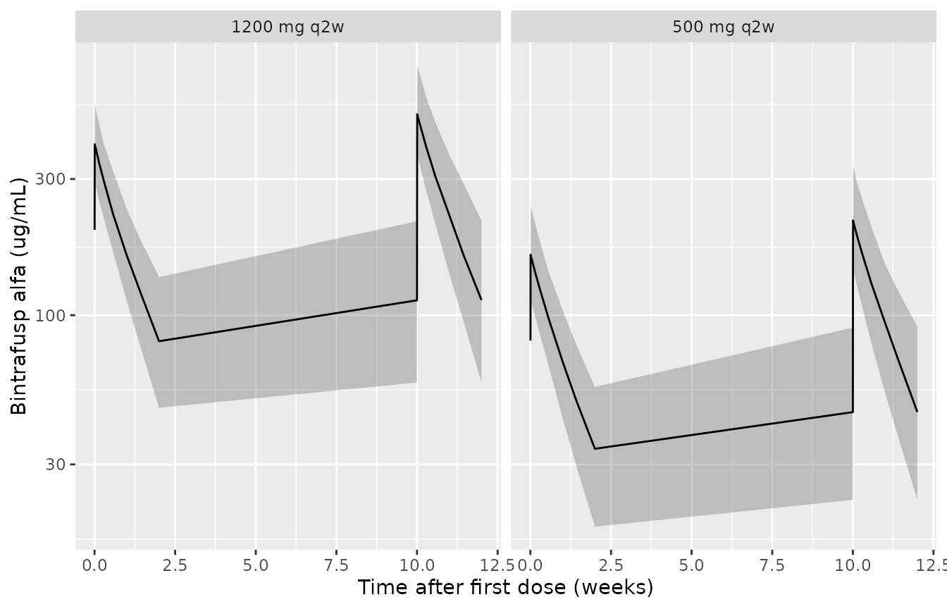
Simulated bintrafusp alfa concentrations after the first and sixth dose (median and 5th-95th percentiles, 200 virtual patients per arm). Compare with Supplementary Figures S1 and S4 of Liu 2023.
PKNCA
nca_conc <- sim_pk |>
  filter(!is.na(Cc)) |>
  select(id, time, Cc, treatment)
nca_dose <- events_pk |>
  filter(evid == 1) |>
  select(id, time, amt, treatment)
intervals <- data.frame(
  start = c(0, 5 * tau),
  end = c(tau, 6 * tau),
  cmax = TRUE,
  tmax = TRUE,
  clast.obs = TRUE,
  auclast = TRUE
)
nca_res <- PKNCA::pk.nca(PKNCA::PKNCAdata(
  PKNCA::PKNCAconc(nca_conc, Cc ~ time | treatment + id),
  PKNCA::PKNCAdose(nca_dose, amt ~ time | treatment + id),
  intervals = intervals
))
nca_tab <- as.data.frame(nca_res) |>
  filter(PPTESTCD %in% c("cmax", "clast.obs", "auclast")) |>
  mutate(Dose = ifelse(start == 0, "First dose", "Sixth dose")) |>
  group_by(treatment, Dose, PPTESTCD) |>
  summarise(median = signif(median(PPORRES), 3), .groups = "drop") |>
  pivot_wider(names_from = PPTESTCD, values_from = median)
nca_tab |>
  rename(
    "Arm" = treatment,
    "Cmax (ug/mL)" = cmax,
    "C at 336 h, trough (ug/mL)" = clast.obs,
    "AUC0-336 h (h*ug/mL)" = auclast
  ) |>
knitr::kable(caption = "Median simulated NCA parameters over the first and sixth dosing intervals.")| Arm | Dose | AUC0-336 h (h*ug/mL) | C at 336 h, trough (ug/mL) | Cmax (ug/mL) |
|---|---|---|---|---|
| 1200 mg q2w | First dose | 61500 | 81.0 | 397 |
| 1200 mg q2w | Sixth dose | 83800 | 113.0 | 506 |
| 500 mg q2w | First dose | 26300 | 34.0 | 163 |
| 500 mg q2w | Sixth dose | 35100 | 45.8 | 215 |
Liu 2023 reports no NCA table, so the check is structural. At steady state the typical-value AUC over one dosing interval must equal Dose / CL, and the PK is dose-proportional (Results: ‘dose-proportional PKs and close to complete separation of systemic exposures between the two dose groups’).
# Typical values: omega zeroed, so the note about a multi-subject solve
# without omega is expected.
typ <- suppressWarnings(rxode2::rxSolve(rxode2::zeroRe(mod_pk, "omega"),
  events = events_pk |> filter(id %in% c(1, n_per_arm + 1)),
  keep = "treatment", returnType = "data.frame"
), classes = "warning")
#> ℹ parameter labels from comments will be replaced by 'label()'
#> ℹ omega/sigma items treated as zero: 'etalcl', 'etalvc', 'etaRUV'
typ_nca <- PKNCA::pk.nca(PKNCA::PKNCAdata(
  PKNCA::PKNCAconc(typ |> select(id, time, Cc, treatment), Cc ~ time | treatment + id),
  PKNCA::PKNCAdose(events_pk |> filter(evid == 1, id %in% c(1, n_per_arm + 1)) |> select(id, time, amt, treatment), amt ~ time | treatment + id),
  intervals = data.frame(start = 5 * tau, end = 6 * tau, auclast = TRUE)
))
auc_ss <- as.data.frame(typ_nca) |>
  filter(PPTESTCD == "auclast") |>
  mutate(dose = ifelse(treatment == "500 mg q2w", 500, 1200), expected = dose / 0.0143,
         pct_diff = 100 * (PPORRES / expected - 1))
knitr::kable(auc_ss |> select(treatment, PPORRES, expected, pct_diff) |>
  rename("Arm" = treatment, "Typical AUCtau,ss (h*ug/mL)" = PPORRES, "Dose / CL" = expected, "% difference" = pct_diff),
digits = 2)| Arm | Typical AUCtau,ss (h*ug/mL) | Dose / CL | % difference |
|---|---|---|---|
| 1200 mg q2w | 84008.09 | 83916.08 | 0.11 |
| 500 mg q2w | 35003.37 | 34965.03 | 0.11 |
Tumour growth inhibition model
The TGI time axis starts at the screening scan, where the baseline
SLD (IBASE) is estimated; drug-induced shrinkage starts at the first
dose, T_SCAN_TO_DOSE later. The cohort uses the mean
screening-to-first-dose interval of 17.6 days (2.51 weeks) for every
patient.
mod_tgi <- readModelDb("Liu_2023_bintrafuspAlfa_tgi")
t_scan <- 17.6 / 7
tgi_times <- seq(0, 60, by = 0.5)
events_tgi <- expand.grid(id = 1:200, time = tgi_times) |>
  mutate(evid = 0L, cmt = "tumor_size", T_SCAN_TO_DOSE = t_scan) |>
  arrange(id, time)
rxode2::rxSetSeed(20232)
sim_tgi <- rxode2::rxSolve(mod_tgi, events = events_tgi, returnType = "data.frame")
#> ℹ parameter labels from comments will be replaced by 'label()'
sim_tgi |>
  group_by(time) |>
  summarise(
    Q05 = quantile(tumor_size, 0.05), Q50 = median(tumor_size), Q95 = quantile(tumor_size, 0.95),
    .groups = "drop"
  ) |>
  ggplot(aes(time - t_scan, Q50)) +
  geom_ribbon(aes(ymin = Q05, ymax = Q95), alpha = 0.25) +
  geom_line() +
  geom_vline(xintercept = 0, linetype = 2) +
  labs(x = "Time after first dose (weeks)", y = "Sum of longest diameters (mm)")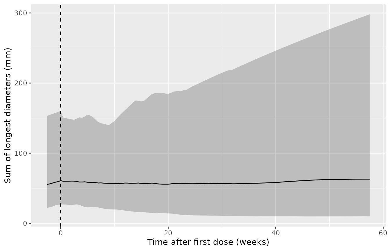
Simulated SLD of target lesions versus time after the first dose (median and 5th-95th percentiles of the individual predictions, 200 virtual patients). Compare with Supplementary Figure S5 of Liu 2023, whose observed median is about 58 mm before treatment, rises to about 63 mm at week 6 and settles near 40 mm from week 30.
The observed medians of Figure S5 come from patients still on study, and patients who progress drop out of the tumour-size data, so the simulated median (which keeps every patient) need not follow the late observed median.
The typical-value trajectory has a closed form. Before the first dose
the SLD grows linearly, IBASE + KG t; afterwards, with
A(T) = (kD / lambda)(1 - exp(-lambda T)),
SLD(T) = exp(-A(T)) [SLD(T0) + KG * integral_0^T exp(A(u)) du].
typ_tgi <- rxode2::rxSolve(rxode2::zeroRe(mod_tgi, "omega"), events = events_tgi |> filter(id == 1), returnType = "data.frame")
#> ℹ parameter labels from comments will be replaced by 'label()'
#> ℹ omega/sigma items treated as zero: 'etalrbase', 'etalkg', 'etalkd', 'etaRUV'
kg <- 1.43; kd <- 0.0306; lam <- 0.00559; ibase <- 56.3
A <- function(T) kd / lam * (1 - exp(-lam * T))
closed <- vapply(typ_tgi$time, function(tt) {
  if (tt <= t_scan) return(ibase + kg * tt)
  T <- tt - t_scan
  exp(-A(T)) * (ibase + kg * t_scan + kg * integrate(function(u) exp(A(u)), 0, T)$value)
}, numeric(1))
rel_err <- abs(typ_tgi$tumor_size / closed - 1)
c(max_rel_err = max(rel_err), nadir_mm = min(closed[typ_tgi$time > t_scan]),
  nadir_week_after_dose = typ_tgi$time[which.min(ifelse(typ_tgi$time > t_scan, closed, Inf))] - t_scan)
#>           max_rel_err              nadir_mm nadir_week_after_dose
#>          1.369817e-07          5.502076e+01          2.898571e+01
# Same parameters on both sides: the difference is LSODA tolerance only.
stopifnot(max(rel_err) < 1e-4)
Multistate model
All patients start in stable disease (S1) at the first dose.
Transitions are forward only: S1 to response (S2), progression (S3),
unknown (S4), dropout (S5) or death (S6); S2 to S3, S4 or S6; S3 to S5
or S6; S4 to S5 or S6. Each ODE state is the probability of occupying
that state, so a solve without any data returns the marginal
state-occupancy curves of a patient population. When fitting, the source
resets all states after each observation to the observed state; the
shipped model reproduces that with evid = 5 replace
events.
The models have no between-subject variability, so the validation below is deterministic. Each arm is a mixture of patients with and without baseline metastases in the Table 1 proportions (33 of 40 at 500 mg, 32 of 40 at 1200 mg); age only moves the very small background mortality and is set to the arm mean.
mod_ms <- readModelDb("Liu_2023_bintrafuspAlfa_multistate")
mod_msd <- readModelDb("Liu_2023_bintrafuspAlfa_multistate_dose")
weeks_per_month <- 365.25 / 12 / 7
ms_times <- seq(0, 180, by = 0.25)
grid <- tibble(
  id = 1:4,
  arm = rep(c("500 mg q2w", "1200 mg q2w"), each = 2),
  DOSE_HIGH = rep(c(0, 1), each = 2),
  MET_GE1 = rep(c(0, 1), 2),
  AGE = rep(c(63.9, 62.1), each = 2),
  w = c(7 / 40, 33 / 40, 8 / 40, 32 / 40)
)
events_ms <- tidyr::expand_grid(id = grid$id, time = ms_times) |>
  left_join(grid |> select(id, DOSE_HIGH, MET_GE1, AGE), by = "id") |>
  mutate(evid = 0L, cmt = "s_stable")

# The multistate models have no between-subject variability by design, so
# rxSolve's note about a multi-subject solve without omega is expected.
solve_ms <- function(mod, params = NULL) {
  suppressWarnings(
    rxode2::rxSolve(mod, events = events_ms, params = params, returnType = "data.frame"),
    classes = "warning"
  ) |>
    left_join(grid |> select(id, arm, w), by = "id")
}
arm_mix <- function(d, value) {
  d |>
    mutate(v = {{ value }}) |>
    group_by(arm, time) |>
    summarise(v = sum(w * v), .groups = "drop")
}
The ODE system is checked against its one closed-form piece: S1 is
left only by constant hazards and the Weibull k13, so
P1(t) = exp(-(k12 + k14 + k15 + k16) t - (scale13 t)^shape13 exp(beta (1 - MET_GE1))).
ms_dose <- solve_ms(mod_msd)
p1 <- ms_dose |>
  mutate(closed = exp(-(k12 + k14 + k15 + k16) * time -
    (scale13 * time)^shape13 * exp(-1.430 * (1 - MET_GE1))))
c(max_rel_err_P1 = max(abs(p1$prob_stable_disease / p1$closed - 1)),
  max_mass_balance_err = max(abs(ms_dose$prob_state_sum - 1)))
#>       max_rel_err_P1 max_mass_balance_err
#>         1.126389e-05         6.217249e-15
stopifnot(
  max(abs(p1$prob_stable_disease / p1$closed - 1)) < 1e-3,
  max(abs(ms_dose$prob_state_sum - 1)) < 1e-6
)
State occupancy (Figure 2)
state_labels <- c(
  prob_stable_disease = "Stable disease", prob_tumor_response = "Response",
  prob_progressive_disease = "Progression", prob_unknown_status = "Unknown",
  prob_dropout = "Dropout", prob_death = "Death"
)
ms_dose |>
  select(id, time, arm, w, all_of(names(state_labels))) |>
  pivot_longer(all_of(names(state_labels)), names_to = "state", values_to = "p") |>
  group_by(arm, state, time) |>
  summarise(p = sum(w * p), .groups = "drop") |>
  mutate(state = factor(state_labels[state], levels = state_labels)) |>
  ggplot(aes(time, p, colour = arm)) +
  geom_line() +
  facet_wrap(~state, scales = "free_y") +
  labs(x = "Time after first dose (weeks)", y = "Probability", colour = NULL) +
  theme(legend.position = "bottom")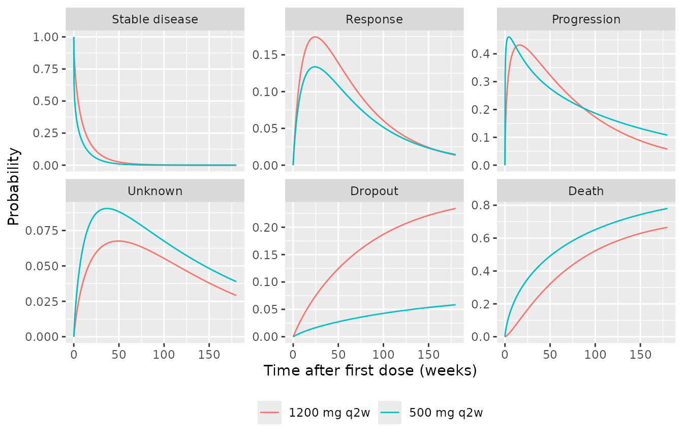
Probability of occupying each state by dose arm (dose-dependent model). Compare with the state-proportion panels of Figure 2 of Liu 2023.
PFS, OS and response by dose (Figure 3)
The end points follow the paper’s definitions (Methods, ‘Derivation of PFS and OS’):
-
PFS: progression is only seen at a tumour
assessment (every 6 weeks in year one, every 12 weeks after), while
death from S1/S2 counts when it happens; transitions to unknown or
dropout censor PFS. Under the model’s Markov assumption, censoring that
is independent of the hazards leaves the event-free curve of a world
without those transitions, so PFS at an assessment is
P1 + P2from a solve with k14, k24 and the dropout hazard switched off. -
OS: time to dropout or death,
1 - P5 - P6. -
Overall response rate: the probability of ever
entering the response state,
integral of k12 * P1 dt, up to 180 weeks of follow-up.
off <- log(1e-12)
ms_pfs <- solve_ms(mod_msd, params = c(
  lk14_500mg = off, lk14_1200mg = off, lk24_500mg = off, lk24_1200mg = off,
  lkdrop_500mg = off, lkdrop_1200mg = off
))
visits <- c(seq(6, 48, by = 6), seq(60, 180, by = 12))
pfs <- arm_mix(ms_pfs, prob_stable_disease + prob_tumor_response) |>
  filter(time %in% visits)
os <- arm_mix(ms_dose, 1 - prob_dropout - prob_death)
orr <- ms_dose |>
  group_by(id, arm, w) |>
  arrange(time, .by_group = TRUE) |>
  summarise(orr = sum(diff(time) * (head(k12 * prob_stable_disease, -1) + tail(k12 * prob_stable_disease, -1)) / 2),
            .groups = "drop") |>
  group_by(arm) |>
  summarise(orr = sum(w * orr))

pfs_step <- bind_rows(
  tibble(arm = unique(pfs$arm), time = 0, v = 1),
  pfs
)
bind_rows(
  pfs_step |> mutate(endpoint = "PFS"),
  os |> mutate(endpoint = "OS")
) |>
  filter(time <= 150) |>
  ggplot(aes(time, 100 * v, colour = arm)) +
  geom_step(data = ~ filter(.x, endpoint == "PFS")) +
  geom_line(data = ~ filter(.x, endpoint == "OS")) +
  facet_wrap(~endpoint) +
  scale_colour_manual(values = c("500 mg q2w" = "red", "1200 mg q2w" = "blue")) +
  labs(x = "Time after first dose (weeks)", y = "Survival (%)", colour = NULL,
       caption = "Replicates the median curves of Figure 3 of Liu 2023 (typical parameters, no parameter uncertainty).") +
  theme(legend.position = "bottom")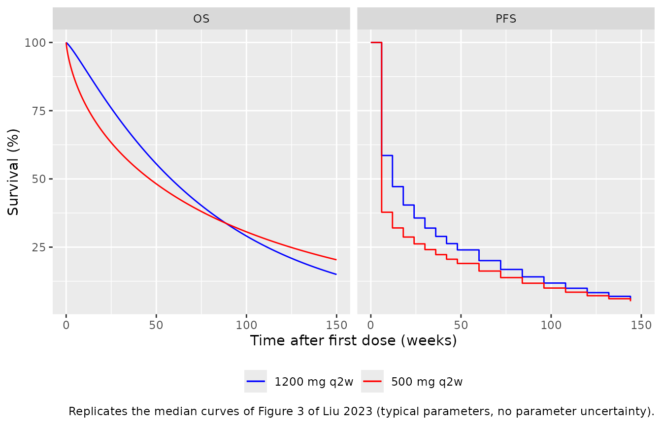
med <- function(d) {
  d |>
    group_by(arm) |>
    summarise(med_wk = min(time[v <= 0.5]))
}
os_med <- os |>
  group_by(arm) |>
  summarise(os_wk = approx(v, time, 0.5)$y)
cmp <- grid |>
  distinct(arm) |>
  left_join(orr, by = "arm") |>
  left_join(med(pfs) |> rename(pfs_wk = med_wk), by = "arm") |>
  left_join(os_med, by = "arm") |>
  mutate(
    pfs_mo = pfs_wk / weeks_per_month,
    os_mo = os_wk / weeks_per_month,
    paper_orr = c(20, 27),
    paper_pfs_mo = c(1.4, 2.6),
    paper_os_mo = c(11.0, 13.7)
  )
cmp |>
  transmute(
    "Arm" = arm,
    "ORR (%)" = round(100 * orr, 1), "Paper ORR (%)" = paper_orr,
    "Median PFS (months)" = round(pfs_mo, 2), "Paper PFS (months)" = paper_pfs_mo,
    "Median OS (months)" = round(os_mo, 1), "Paper OS (months)" = paper_os_mo
  ) |>
knitr::kable(caption = "Typical-parameter predictions versus the median of the 500 simulated trials in Liu 2023 Results (ORR 20% / 27%, PFS 1.4 / 2.6 months, OS 11.0 / 13.7 months).")| Arm | ORR (%) | Paper ORR (%) | Median PFS (months) | Paper PFS (months) | Median OS (months) | Paper OS (months) |
|---|---|---|---|---|---|---|
| 500 mg q2w | 20.5 | 20 | 1.38 | 1.4 | 10.7 | 11.0 |
| 1200 mg q2w | 29.2 | 27 | 2.76 | 2.6 | 13.4 | 13.7 |
stopifnot(
  # The PFS median falls on the first (week 6) and second (week 12) assessment.
  identical(cmp$pfs_wk, c(6, 12)),
  abs(100 * cmp$orr - cmp$paper_orr) < 5,
  abs(cmp$os_mo / cmp$paper_os_mo - 1) < 0.10
)
The paper’s figures are medians over 500 simulated trials that resample the parameters from their sampling-importance-resampling uncertainty, so a typical-parameter prediction need not hit them exactly; ORR, median PFS and median OS all agree within a few percent. Figure 4 (probability that the 1200 mg arm’s median OS exceeds the 500 mg arm’s by at least X months) needs those parameter samples, which are not published, and is not reproduced.
Final model (dose-independent)
The final multistate model pools both arms. Its predictions for the pooled cohort (65 of 80 patients with metastases) should fall between the two arms of the dose-dependent model.
ms_final <- solve_ms(mod_ms)
pooled <- ms_final |>
  filter(id %in% c(1, 2)) |>
  mutate(w = ifelse(MET_GE1 == 1, 65 / 80, 15 / 80), arm = "Pooled (final model)")
os_final <- arm_mix(pooled, 1 - prob_dropout - prob_death) |>
  summarise(os_mo = approx(v, time, 0.5)$y / weeks_per_month)
orr_final <- pooled |>
  group_by(id, w) |>
  arrange(time, .by_group = TRUE) |>
  summarise(orr = sum(diff(time) * (head(k12 * prob_stable_disease, -1) + tail(k12 * prob_stable_disease, -1)) / 2),
            .groups = "drop") |>
  summarise(orr = sum(w * orr))
c(pooled_orr_pct = 100 * orr_final$orr, observed_pooled_orr_pct = (15 + 28) / 2,
  pooled_median_os_mo = os_final$os_mo)
#>          pooled_orr_pct observed_pooled_orr_pct     pooled_median_os_mo
#>                24.44420                21.50000                11.11124
stopifnot(
  os_final$os_mo > min(cmp$os_mo), os_final$os_mo < max(cmp$os_mo),
  abs(100 * orr_final$orr - 21.5) < 5
)
Assumptions and deviations
-
Residual error with a random effect on its
magnitude. Supplementary Table S2 lists, for each of the PK and
tumour-size models, a ‘sigma^2 EPS’ variance (0.260 and 0.0288) next to
the residual-error parameters, and gives each its own shrinkage. The
maintainers read these as between-subject variances of the
residual-error magnitude (
etaRUV), the usual Uppsala parameterisationW * exp(eta) * EPSwith EPS variance fixed to 1: a separately estimated EPS variance on top of estimated proportional and additive SDs would not be identifiable, and two shrinkage values imply two random effects. -
Gompertz-Makeham background mortality. The Appendix
S2 control stream writes
X1 = EXP(BETA*AGE-30). Taken literally the age term vanishes (exp(0.114 * 63 - 30)is about1e-10) and the curve collapses to its constant term. The maintainers read it asEXP(BETA*(AGE-30)), the Missov-Lenart gamma-Gompertz-Makeham hazard with age counted from 30 that the paper cites; the resulting stable-disease-to-death hazard (about 0.0002 per week at age 63) is negligible next to the other transitions either way. The example control stream does not list AGE in$INPUT; baseline age is used. -
Metastasis coding. Supplementary Table S3 codes the
source column as ‘Metastases (0:Yes or 1:No)’. With the coefficient
-1.431 this makes the metastatic majority the reference and raises k13
4.18-fold relative to patients without metastases, as the Results state.
The model uses the canonical
MET_GE1(1 = metastases) and applies the coefficient to1 - MET_GE1. The reverse coding would leave the majority with a 4.18-fold higher hazard and put median PFS in both arms at the first assessment, contrary to the published 1.4 and 2.6 months. - Parameter precision. Table 2 prints most hazards to one or two significant figures (e.g. k24 = 0.002 vs 0.004); those printed values are used. The example control stream in Appendix S2 carries more digits, but its estimates are close to, not equal to, the Table 2 1200 mg column and it is labelled an example, so it is used only for the model structure and the fixed Gompertz-Makeham constants.
-
Placeholder residual. The source fits the
multistate model with the exact categorical likelihood and has no
residual error. A tiny additive error (
addSd = 0.001) onprob_deathlets nlmixr2 accept the model; it is not from the paper. -
Dose-dependent model as a separate file. The
dose-dependent model estimates every transition separately per arm; it
is shipped as its own model, with
DOSE_HIGHselecting the 1200 mg values. It does not interpolate to other doses. - PK infusion duration and dosing cohort. A 1-hour infusion is used (end of infusion is 1 hour after the start of dosing per Supplementary Table S1 and Figure S2). Vp and Q are fixed to Wilkins 2019, as in the source.
- TGI screening interval. Every virtual patient uses the mean screening-to-first-dose interval of 17.6 days; the source range was 1.4-48.4 days.
- No erratum or correction for Liu 2023 was found in Europe PMC as of 2026-10-28.