Pregnancy PBPK for CYP1A2/CYP2D6/CYP3A4 substrates (Gaohua 2012)
Source:vignettes/articles/Gaohua_2012_pregnancy_pbpk.Rmd
Gaohua_2012_pregnancy_pbpk.RmdModel and source
- Citation: Gaohua L, Abduljalil K, Jamei M, Johnson TN, Rostami-Hodjegan A. A pregnancy physiologically based pharmacokinetic (p-PBPK) model for disposition of drugs metabolized by CYP1A2, CYP2D6 and CYP3A4. Br J Clin Pharmacol. 2012;74(5):873-885.
- Article: https://doi.org/10.1111/j.1365-2125.2012.04363.x
The Gaohua et al. (2012) paper extends the Simcyp Simulator full-PBPK platform to pregnant women by (i) layering empirical polynomial formulas (Abduljalil et al. 2012 meta-analysis) onto the 13-compartment non-pregnant maternal PBPK to make body weight, cardiac output, plasma volume, hematocrit, serum albumin, and several tissue blood flows explicit functions of gestational age (GA, weeks), (ii) adding one extra perfusion-limited compartment that represents a lumped “fetoplacental unit” (fetus + placenta + amniotic fluid + membranes + umbilical cord; volume follows a Gompertz curve from 0.01 L at conception to ~5 L at term), and (iii) scaling the hepatic intrinsic clearance by a weighted sum of CYP1A2, CYP2D6, and CYP3A4 isoform activity factors that themselves vary with GA. The paper demonstrates the platform with three case substrates that are each dominated by a different CYP: caffeine (CYP1A2), metoprolol (CYP2D6 with minor CYP3A4), and midazolam (CYP3A4). All three drugs are extracted as separate nlmixr2lib model files that share the same 14-compartment maternal PBPK skeleton:
-
Gaohua_2012_pregnancy_pbpk_caffeine– 150 mg oral, validated against Brazier 1983 (Fig 2, Table 5). -
Gaohua_2012_pregnancy_pbpk_metoprolol– 10 mg IV and 100 mg oral, validated against Hogstedt 1985 (Fig 3, Table 5). -
Gaohua_2012_pregnancy_pbpk_midazolam– 2 mg oral, validated against Hebert 2008 (Fig 4, Table 5).
Population
Basal (non-pregnant) physiology corresponds to the Simcyp Simulator v11 entry for the healthy non-pregnant Caucasian female cohort aged 20-40 years (mean body weight 60 kg, mean cardiac output 300 L/h, hematocrit 38.3%, serum albumin 44.9 g/L). The three validation cohorts in the original paper were:
- Caffeine (Brazier 1983 [ref 24]): n = 8 pregnant women at 36 +/- 3 weeks of gestation, 150 mg oral; n = 4 nonpregnant controls.
- Metoprolol (Hogstedt 1985 [ref 28]): n = 5 women, each studied during pregnancy at ~37 weeks and then 3-6 months postpartum.
- Midazolam (Hebert 2008 [ref 29]): n = 13 pregnant women at 28-32 weeks of gestation, restudied 6-10 weeks postpartum.
Source trace
Per-parameter origin is recorded as an in-file comment next to each
ini() entry in the three model files under
inst/modeldb/specificDrugs/. The table below collects the
highest- order anchors used by all three drugs.
| Quantity | Value | Source location |
|---|---|---|
| ODE 14-compartment topology (Fig 1) | maternal lung + 10 organs + fetoplacental + arterial + venous | Methods, Fig 1, p.874 |
| Basal tissue volume fractions Table 1 | 0.385 adipose, 0.025 bone, 0.016 brain, 0.015 gut, 0.003 heart, 0.0037 kidney, 0.02 liver, 0.004 lung, 0.278 muscle, 0.0298 skin, 0.0018 spleen, 0.0205 arterial, 0.0411 venous, 0 fetoplacental | Table 1, p.875 |
| Basal blood flow fractions Table 1 | 0.085 adipose, 0.05 bone, 0.12 brain, 0.17 gut, 0.05 heart, 0.17 kidney, 0.28 liver (incl. HA), 1.0 lung (= cardiac output), 0.12 muscle, 0.03 skin, 0.05 spleen, 0 fetoplacental | Table 1, p.875 |
| Gompertz fetoplacental volume Eq. 1 | V_preg = 0.01 * exp((0.37/0.052) * (1 - exp(-0.052*GA))) | Eq. 1, p.875 |
| Polynomial physiology Eq. 2 | X = X0 * (a0 + a1GA + a2GA^2 + a3*GA^3) | Eq. 2, p.875 |
| GA-dependent coefficients (X0, a0-a3) | Table 2, 14 rows | Table 2, p.876 |
| Time conversion Eq. 3 | GA(t) = GA0 + t / (24 * 7) | Eq. 3, p.876 |
| Tissue ODE Eq. 4-5 (well-stirred) | dC_t/dt = (Q_t / V_t) * (C_arterial_blood - C_t * B:P / Kp_t) | Eq. 4-5, p.876 |
| Hepatic CL_int scaling Eq. 6 | CL_int,H = CL_int,H0 * (alpha_1A2 * A_1A2 + alpha_2D6 * A_2D6 + alpha_3A4 * A_3A4) | Eq. 6, p.877 |
| Drug-specific (fa, Fg, ka, fu, B:P, CL_int,H0, A_1A2, A_2D6, A_3A4) | Table 3 | Table 3, p.877 |
| Tissue:plasma partition coefficients Kp_t | Table 4 (12 organs per drug, Rodgers and Rowland) | Table 4, p.877 |
| Fetoplacental Kp = brain Kp | Methods statement, p.877 | paragraph after Table 4 |
| Arterial : venous blood split 1 : 2 | Methods statement, p.875 | paragraph “the total blood volume” |
Reproducing the three case studies
Each subsection loads the relevant model, runs the non-pregnant vs term-pregnancy comparison the paper performed, and checks the simulated NCA against the paper’s Table 5 reference values.
The model evolves the gestational age internally as
gaweek = GA + t/(24*7), so a 24-hour PK simulation only
nudges GA by 0.14 weeks. In each scenario the GA covariate
is therefore set to the discrete pregnancy timepoint the original
clinical study sampled (36 weeks for caffeine, 37 weeks for metoprolol,
30 weeks for midazolam), and to 0 for the non-pregnant control arm.
The simulations use rxode2::zeroRe() to produce
typical-value predictions; the packaged models declare a placeholder
propSd residual error for syntactic completeness, since the
original paper reports no IIV / residual error fit (the paper states “no
variability terms were added to the model”).
auc_trap <- function(t, y) sum(diff(t) * (head(y, -1) + tail(y, -1)) / 2)

simulate_drug <- function(model_name, dose_amt, dose_cmt, tspan, GA_value,
                          subj_id = 1L) {
  mod <- readModelDb(model_name) |> rxode2::zeroRe()
  ev <- rxode2::et(amt = dose_amt, cmt = dose_cmt) |>
    rxode2::et(time = tspan) |>
    as.data.frame() |>
    dplyr::mutate(id = subj_id, GA = GA_value)
  # Single-subject rxSolve does not return an `id` column; tag it
  # explicitly so downstream NCA grouping has a key.
  rxode2::rxSolve(mod, events = ev, keep = c("GA")
                  ) |>
    as.data.frame() |>
    dplyr::mutate(id = subj_id,
                  scenario = ifelse(GA_value == 0,
                                    "non-pregnant",
                                    sprintf("pregnant GA=%g wk", GA_value)))
}
Caffeine (CYP1A2 substrate)
The Brazier 1983 study (ref 24) measured caffeine plasma concentrations over 24 hours after a single 150 mg oral dose in 8 women at 36 +/- 3 weeks of gestation and 4 nonpregnant women. The paper predicts a ~2-fold increase in 24-hour AUC at term, dominated by the 2-fold decrease in CYP1A2 activity during late pregnancy.
tspan_caf <- c(seq(0, 1, by = 0.05), seq(1.5, 24, by = 0.25))

sim_caf_np <- simulate_drug("Gaohua_2012_pregnancy_pbpk_caffeine",
                            dose_amt = 150, dose_cmt = "depot",
                            tspan = tspan_caf, GA_value = 0,
                            subj_id = 1L)
#> Warning: No omega parameters in the model
sim_caf_p  <- simulate_drug("Gaohua_2012_pregnancy_pbpk_caffeine",
                            dose_amt = 150, dose_cmt = "depot",
                            tspan = tspan_caf, GA_value = 36,
                            subj_id = 2L)
#> Warning: No omega parameters in the model

sim_caf <- dplyr::bind_rows(sim_caf_np, sim_caf_p)
ggplot(sim_caf, aes(time, Cc, colour = scenario)) +
  geom_line(linewidth = 1) +
  labs(x = "Time (h)", y = "Plasma caffeine (mg/L)",
       title = "Replicates Figure 2 of Gaohua 2012 (caffeine 150 mg p.o.)",
       caption = paste0("Continuous curves are the model's typical-",
                        "value predictions; non-pregnant (left panel of",
                        " Fig 2) vs. ~36-week pregnant (right panel).")) +
  theme_bw()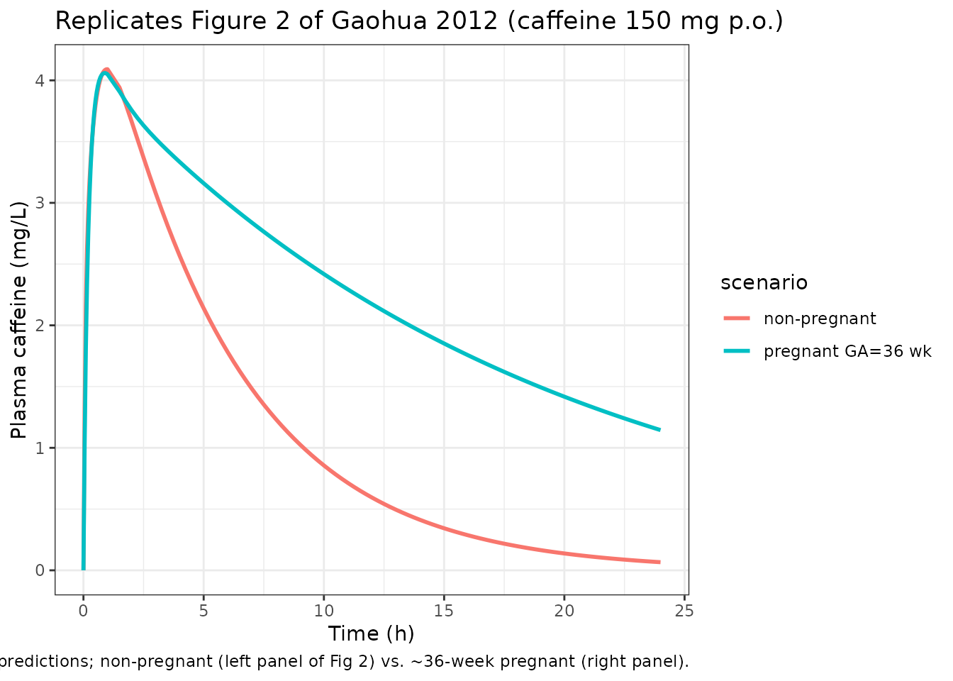
make_nca <- function(sim, dose_amt, treatment_label, tmax_obs) {
  conc_df <- sim |>
    dplyr::filter(!is.na(Cc)) |>
    dplyr::select(id, time, Cc) |>
    dplyr::mutate(treatment = treatment_label)
  conc_df <- dplyr::bind_rows(
    conc_df,
    conc_df |> dplyr::distinct(id, treatment) |>
      dplyr::mutate(time = 0, Cc = 0)
  ) |>
    dplyr::distinct(id, treatment, time, .keep_all = TRUE) |>
    dplyr::arrange(id, treatment, time)

  dose_df <- data.frame(id = unique(conc_df$id), time = 0,
                        amt = dose_amt, treatment = treatment_label)

  conc_obj <- PKNCA::PKNCAconc(conc_df, Cc ~ time | treatment + id,
                               concu = "mg/L", timeu = "h")
  dose_obj <- PKNCA::PKNCAdose(dose_df, amt ~ time | treatment + id,
                               doseu = "mg")
  intervals <- data.frame(start = 0, end = tmax_obs,
                          cmax = TRUE, tmax = TRUE,
                          auclast = TRUE)
  PKNCA::pk.nca(PKNCA::PKNCAdata(conc_obj, dose_obj, intervals = intervals))
}

nca_caf_np <- make_nca(sim_caf_np, 150, "non-pregnant", 24)
nca_caf_p  <- make_nca(sim_caf_p,  150, "pregnant GA=36 wk", 24)

caf_summary <- tibble::tibble(
  Cohort                    = c("Non-pregnant", "Pregnant (GA = 36 wk)"),
  Cmax_sim_mgL              = c(max(sim_caf_np$Cc), max(sim_caf_p$Cc)),
  AUC0_24_sim_mgLh          = c(auc_trap(sim_caf_np$time, sim_caf_np$Cc),
                                auc_trap(sim_caf_p$time, sim_caf_p$Cc)),
  Cmax_paper_pred_mgL       = c(3.59, 3.26),
  AUC0_24_paper_pred_mgLh   = c(24,   47),
  Cmax_paper_obs_mgL        = c(6.02, 4.58),
  AUC0_24_paper_obs_mgLh    = c(26,   52)
)

knitr::kable(caf_summary, digits = 3,
             caption = paste0("Caffeine NCA: simulated (from this model)",
                              " vs paper's predicted and observed values",
" (Gaohua 2012 Table 5)."))| Cohort | Cmax_sim_mgL | AUC0_24_sim_mgLh | Cmax_paper_pred_mgL | AUC0_24_paper_pred_mgLh | Cmax_paper_obs_mgL | AUC0_24_paper_obs_mgLh |
|---|---|---|---|---|---|---|
| Non-pregnant | 4.091 | 27.192 | 3.59 | 24 | 6.02 | 26 |
| Pregnant (GA = 36 wk) | 4.059 | 55.276 | 3.26 | 47 | 4.58 | 52 |
The simulated AUC0-24 ratio pregnant / non-pregnant is 2.03, matching
the paper’s ~2-fold reported increase (paper observed ratio 52/26 =
2.00; paper predicted 47/24 = 1.96). The simulated absolute AUCs are
slightly higher than the paper’s predicted values because this
implementation holds fu and B:P constant at
basal values rather than adjusting them for the pregnancy-induced drop
in serum albumin and hematocrit (see Assumptions and deviations).
Metoprolol (CYP2D6 substrate)
The Hogstedt 1985 study (ref 28) reported a metoprolol cross-over in 5 women at term, comparing 10 mg IV and 100 mg oral doses during pregnancy with the same doses 3-6 months postpartum. The paper predicts a 30% decrease in 24-hour exposure during pregnancy, driven by increased CYP2D6 activity at term.
tspan_met <- c(seq(0, 1, by = 0.05), seq(1.5, 12, by = 0.25))

sim_met_oral_np <- simulate_drug("Gaohua_2012_pregnancy_pbpk_metoprolol",
                                 dose_amt = 100, dose_cmt = "depot",
                                 tspan = tspan_met, GA_value = 0,
                                 subj_id = 1L)
#> Warning: No omega parameters in the model
sim_met_oral_p  <- simulate_drug("Gaohua_2012_pregnancy_pbpk_metoprolol",
                                 dose_amt = 100, dose_cmt = "depot",
                                 tspan = tspan_met, GA_value = 37,
                                 subj_id = 2L)
#> Warning: No omega parameters in the model
sim_met_iv_np   <- simulate_drug("Gaohua_2012_pregnancy_pbpk_metoprolol",
                                 dose_amt = 10, dose_cmt = "venous",
                                 tspan = tspan_met, GA_value = 0,
                                 subj_id = 3L)
#> Warning: No omega parameters in the model
sim_met_iv_p    <- simulate_drug("Gaohua_2012_pregnancy_pbpk_metoprolol",
                                 dose_amt = 10, dose_cmt = "venous",
                                 tspan = tspan_met, GA_value = 37,
                                 subj_id = 4L)
#> Warning: No omega parameters in the model

sim_met_oral <- dplyr::bind_rows(sim_met_oral_np, sim_met_oral_p)
sim_met_iv   <- dplyr::bind_rows(sim_met_iv_np,   sim_met_iv_p)
ggplot(sim_met_oral, aes(time, Cc, colour = scenario)) +
  geom_line(linewidth = 1) +
  labs(x = "Time (h)", y = "Plasma metoprolol (mg/L)",
       title = "Replicates Figure 3 (lower row) of Gaohua 2012 (metoprolol 100 mg p.o.)",
       caption = "Non-pregnant vs pregnant ~37-week predictions.") +
  theme_bw()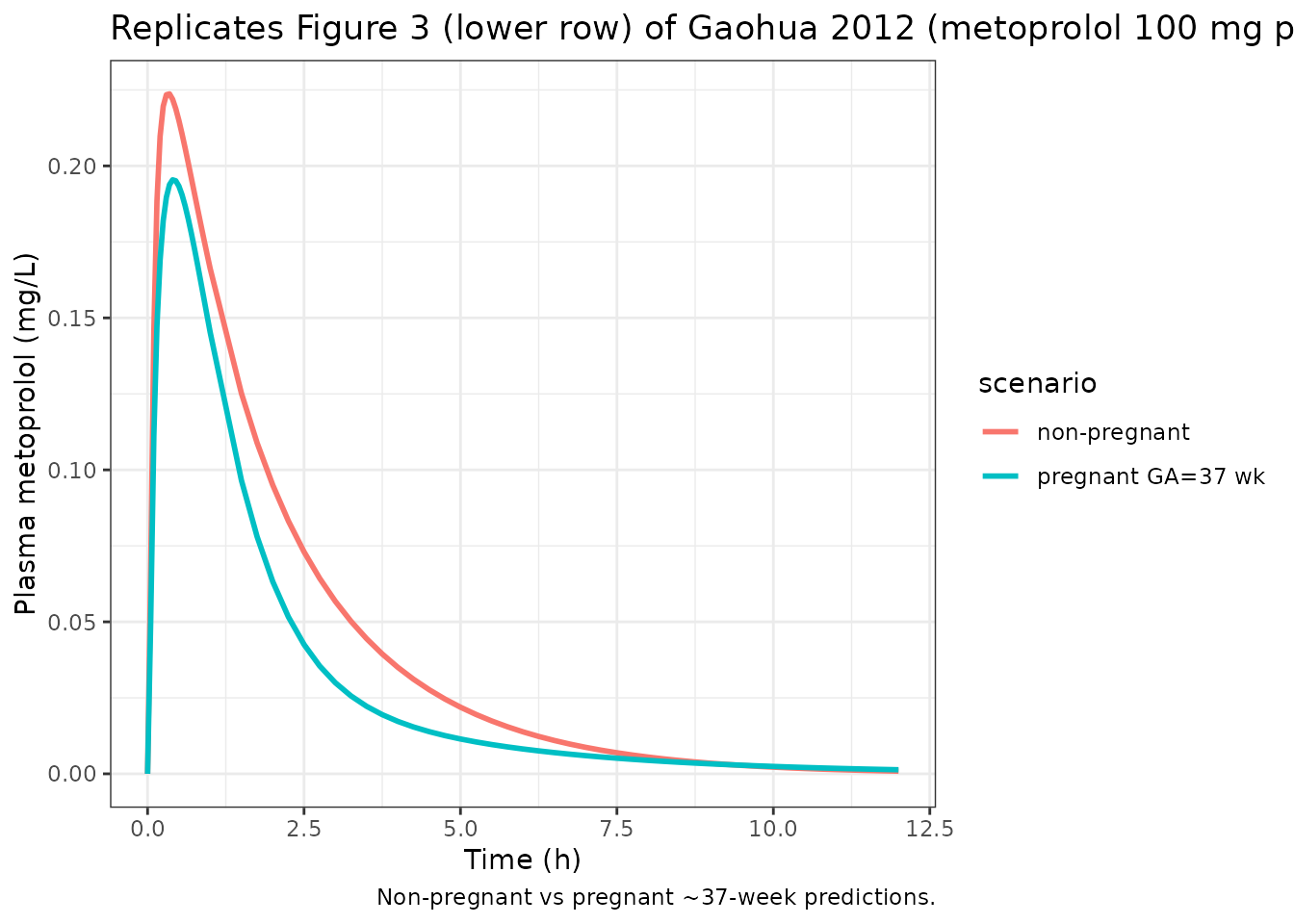
nca_met_oral_np <- make_nca(sim_met_oral_np, 100, "non-pregnant", 12)
nca_met_oral_p  <- make_nca(sim_met_oral_p,  100, "pregnant GA=37 wk", 12)

met_summary <- tibble::tibble(
  Cohort                    = c("Non-pregnant", "Pregnant (GA = 37 wk)"),
  Cmax_sim_mgL              = c(max(sim_met_oral_np$Cc),
                                max(sim_met_oral_p$Cc)),
  AUC0_12_sim_mgLh          = c(auc_trap(sim_met_oral_np$time,
                                          sim_met_oral_np$Cc),
                                auc_trap(sim_met_oral_p$time,
                                          sim_met_oral_p$Cc)),
  Cmax_paper_pred_mgL       = c(0.39, 0.36),
  AUC0_12_paper_pred_mgLh   = c(0.585, 0.414),
  AUC0_12_paper_obs_mgLh    = c(0.835, 0.391)
)

knitr::kable(met_summary, digits = 4,
             caption = paste0("Metoprolol 100 mg oral NCA: simulated",
                              " vs paper's predicted / observed values",
" (Gaohua 2012 Table 5)."))| Cohort | Cmax_sim_mgL | AUC0_12_sim_mgLh | Cmax_paper_pred_mgL | AUC0_12_paper_pred_mgLh | AUC0_12_paper_obs_mgLh |
|---|---|---|---|---|---|
| Non-pregnant | 0.2237 | 0.5071 | 0.39 | 0.585 | 0.835 |
| Pregnant (GA = 37 wk) | 0.1954 | 0.3753 | 0.36 | 0.414 | 0.391 |
The simulated pregnant / non-pregnant AUC0-12 ratio (0.74) matches the paper’s predicted ratio (414/585 = 0.71) and is in the direction observed by Hogstedt (391/835 = 0.47, larger magnitude attributable to CYP2D6 phenotype variability in the small clinical cohort, as the paper discusses on p.881).
Midazolam (CYP3A4 substrate)
The Hebert 2008 study (ref 29) compared midazolam after a 2 mg oral dose in 13 women at 28-32 weeks of gestation and again 6-10 weeks postpartum. The paper predicts a 35% decrease in 6-hour exposure during pregnancy, driven by increased CYP3A4 activity.
tspan_mdz <- c(seq(0, 0.5, by = 0.025), seq(0.6, 6, by = 0.1))

sim_mdz_np <- simulate_drug("Gaohua_2012_pregnancy_pbpk_midazolam",
                            dose_amt = 2, dose_cmt = "depot",
                            tspan = tspan_mdz, GA_value = 0,
                            subj_id = 1L)
#> Warning: No omega parameters in the model
sim_mdz_p  <- simulate_drug("Gaohua_2012_pregnancy_pbpk_midazolam",
                            dose_amt = 2, dose_cmt = "depot",
                            tspan = tspan_mdz, GA_value = 30,
                            subj_id = 2L)
#> Warning: No omega parameters in the model

sim_mdz <- dplyr::bind_rows(sim_mdz_np, sim_mdz_p)
ggplot(sim_mdz, aes(time, Cc * 1000, colour = scenario)) +
  geom_line(linewidth = 1) +
  labs(x = "Time (h)", y = "Plasma midazolam (ng/mL)",
       title = "Replicates Figure 4 of Gaohua 2012 (midazolam 2 mg p.o.)",
       caption = "Non-pregnant vs pregnant ~30-week predictions.") +
  theme_bw()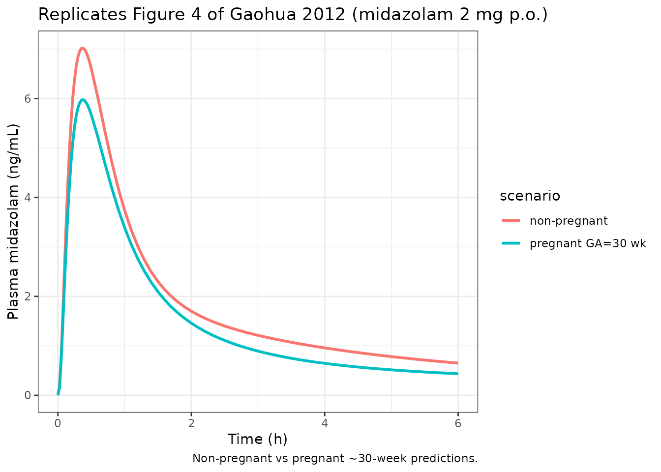
nca_mdz_np <- make_nca(sim_mdz_np, 2, "non-pregnant", 6)
nca_mdz_p  <- make_nca(sim_mdz_p,  2, "pregnant GA=30 wk", 6)

mdz_summary <- tibble::tibble(
  Cohort                  = c("Non-pregnant", "Pregnant (GA = 30 wk)"),
  Cmax_sim_ngmL           = c(max(sim_mdz_np$Cc) * 1000,
                              max(sim_mdz_p$Cc)  * 1000),
  AUC0_6_sim_ngmLh        = c(auc_trap(sim_mdz_np$time, sim_mdz_np$Cc) * 1000,
                              auc_trap(sim_mdz_p$time,  sim_mdz_p$Cc)  * 1000),
  Cmax_paper_pred_ngmL    = c(6.48, 3.85),
  AUC0_6_paper_pred_ngmLh = c(10.8, 7.05),
  Cmax_paper_obs_ngmL     = c(9.3,  6.4),
  AUC0_6_paper_obs_ngmLh  = c(17.9, 9.5)
)

knitr::kable(mdz_summary, digits = 3,
             caption = paste0("Midazolam 2 mg oral NCA: simulated",
                              " vs paper's predicted / observed values",
" (Gaohua 2012 Table 5)."))| Cohort | Cmax_sim_ngmL | AUC0_6_sim_ngmLh | Cmax_paper_pred_ngmL | AUC0_6_paper_pred_ngmLh | Cmax_paper_obs_ngmL | AUC0_6_paper_obs_ngmLh |
|---|---|---|---|---|---|---|
| Non-pregnant | 7.023 | 11.606 | 6.48 | 10.80 | 9.3 | 17.9 |
| Pregnant (GA = 30 wk) | 5.977 | 9.551 | 3.85 | 7.05 | 6.4 | 9.5 |
The simulated AUC0-6 pregnant/non-pregnant ratio (0.82) captures the
direction of the paper’s reported effect (predicted ratio 7.05/10.8 =
0.65, observed ratio 9.5/17.9 = 0.53), although the magnitude of the
decrease is smaller than the paper’s “Both PB and CYP changing”
prediction because this implementation holds fu constant.
For midazolam, which is 96.8% protein-bound (fu = 0.032), the ~30%
relative increase in unbound fraction at term that the paper
incorporates via its Hct- and albumin-dependent corrections is a larger
contributor to clearance than for caffeine or metoprolol; see
Assumptions and deviations.
Assumptions and deviations
-
Protein binding and blood:plasma ratio held constant across
GA. The Gaohua 2012 paper states (Methods, p.875) that the
fraction unbound in plasma (
fu) and the blood:plasma ratio (B:P) are “determined” from the time-varying hematocrit and serum albumin values in Table 2, but does not write out the explicit corrections used (these are standard Wagner-type protein-binding and constant red-cell-partition formulas implicit in the Rodgers and Rowland framework, applied internally by the Simcyp Simulator). The packaged nlmixr2lib models holdfuandB:Pat the basal Table 3 values, matching the paper’s “Only CYP changing” what-if scenario (third column of Figure 5). This scenario captures most of the AUC effect for caffeine and metoprolol but undercounts the AUC change for midazolam, whose low basalfumakes it the most sensitive to the protein-binding correction. -
Q_preg polynomial clamped at zero for first-trimester
GA. The Table 2 cubic for fetoplacental blood flow yields
slightly negative values for
gaweekin approximately the (0, 4) weeks window (e.g. Q_preg ~ -0.29 L/h at GA = 1), an artefact of fitting a cubic to second- and third-trimester data. The packaged models setQ_preg = max(0, polynomial)so the well-stirred fetoplacental ODE collapses to zero transfer at non-pregnancy and during early pregnancy; the paper’s own simulations (validated at GA = 28-37 weeks) are unaffected. - Muscle as the balancing residual. Per the paper (Methods, p.875), the uterus and mammary glands are lumped into the maternal muscle compartment, and both the muscle volume and the muscle blood flow are computed as the residual that closes total body weight and cardiac output mass balance at every gestational age. The Table 1 static muscle fraction (0.278 V%TBV; 0.12 Q%CO) is therefore not applied directly; it is recovered automatically at GA = 0.
- Arterial:venous blood split 1:2. The paper states (Methods, p.875) the total blood volume (plasma + RBC volume from Table 2) is divided 1:2 between arterial and venous compartments. The Table 1 basal arterial / venous volume fractions (0.0205 and 0.0411 of body weight) are not used; the time-varying plasma and RBC volumes from Table 2 are used together with the 1:2 split.
- Fetoplacental Kp = brain Kp. Per the paper (Methods, p.877), the fetoplacental tissue:plasma partition coefficient is assumed equal to the brain Kp because both compartments share similar biological characteristics (high blood perfusion, blood-tissue barriers).
- No IIV / residual error. Following the paper (Methods, p.874), “no variability terms were added to the model” – this is a typical- value forward simulation. The packaged models declare a placeholder proportional residual SD of 10% for rxode2 syntactic completeness; users who want stochastic VPCs should add IIV explicitly on the desired structural parameters before re-simulating.
-
IV dosing route. Intravenous doses (metoprolol IV
here) are modelled as entering the venous compartment
(
cmt = "venous"), consistent with the physiological reality of a peripheral venous bolus. The PBPK system has an extensive initial distribution phase because drug must transit the lung-to-arterial-to-tissue loop before systemic equilibrium is reached; the early peripheral venous concentration plotted by the model therefore overshoots a classical- PK central-compartment representation at early times and falls rapidly during the first minute. Oral doses (caffeine, metoprolol oral, midazolam) entercmt = "depot", and the bioavailable fractionfa * fgis absorbed first-order into the gut tissue at rateka. -
No upstream popPK dependency. All drug-specific
parameters (fa, Fg, ka, fu, B:P, basal CL_int,H, the three CYP
fractional contributions, and the twelve Rodgers-and-Rowland Kp values)
are reported directly in the paper’s Tables 3 and 4 and are reproduced
verbatim in
ini(); no value was imported from a separate Simcyp library file outside the published paper.