Myostatin / activin inhibitors for Duchenne muscular dystrophy, QSP (Nguyen 2020)
Source:vignettes/articles/Nguyen_2020_myostatin_activin_dmd_qsp.Rmd
Nguyen_2020_myostatin_activin_dmd_qsp.RmdModel and source
Nguyen et al. (2020) built a quantitative systems pharmacology (QSP) model of the myostatin / activin A / ActRIIB axis to support the development of FS-EEE-Fc, an engineered follistatin-Fc fusion protein that neutralises both myostatin and activin A, for Duchenne muscular dystrophy (DMD). The same model structure is parameterised for four compounds in humans and for FS-EEE-Fc in three preclinical species. Each parameterisation is packaged as its own model file:
| Model | Compound | Species | Parameters | Sub-models |
|---|---|---|---|---|
Nguyen_2020_fseeefc_qsp |
FS-EEE-Fc | human (projection) | Tables 1-2 | PK, ligands, muscle, FSH |
Nguyen_2020_taldefgrobepAlfa_qsp |
anti-myostatin adnectin BMS-986089 (taldefgrobep alfa) | human | Tables 1-2 | PK, ligands, muscle, FSH |
Nguyen_2020_ramatercept_qsp |
ACE-031 (ramatercept, ActRIIB-Fc) | human | Tables 1-2 | PK, ligands, muscle, FSH |
Nguyen_2020_domagrozumab_qsp |
domagrozumab (PF-06252616) | human | Tables 1-2 | PK (IV), ligands, muscle, FSH |
Nguyen_2020_fseeefc_mouse_qsp |
FS-EEE-Fc | mouse | Tables S3-S4 | PK (IV), ligands, muscle |
Nguyen_2020_fseeefc_rat_qsp |
FS-EEE-Fc | ovariectomised rat | Tables S3-S4 | PK (IV), ligands, FSH |
Nguyen_2020_fseeefc_monkey_qsp |
FS-EEE-Fc | cynomolgus monkey | Tables S3-S4 | PK, ligands |
model_names <- c(
  fseeefc = "Nguyen_2020_fseeefc_qsp",
  adnectin = "Nguyen_2020_taldefgrobepAlfa_qsp",
  ace031 = "Nguyen_2020_ramatercept_qsp",
  domagrozumab = "Nguyen_2020_domagrozumab_qsp",
  mouse = "Nguyen_2020_fseeefc_mouse_qsp",
  rat = "Nguyen_2020_fseeefc_rat_qsp",
  monkey = "Nguyen_2020_fseeefc_monkey_qsp"
)
mods <- lapply(model_names, function(nm) rxode2::rxode2(readModelDb(nm)))- Citation: Nguyen HQ, Iskenderian A, Ehmann D, Jasper P, Zhang Z, Rong H, Welty D, Narayanan R. Leveraging Quantitative Systems Pharmacology Approach into Development of Human Recombinant Follistatin Fusion Protein for Duchenne Muscular Dystrophy. CPT Pharmacometrics Syst Pharmacol. 2020;9(6):342-352. doi:10.1002/psp4.12518. Model equations from the deposited R Markdown (run_QSPmodel.Rmd, Supplementary Information).
- Article: https://doi.org/10.1002/psp4.12518
- Open access at Europe PMC: https://europepmc.org/article/PMC/PMC7306616
Human FS-EEE-Fc. QSP. Myostatin / activin A / ActRIIB systems-pharmacology model for the engineered follistatin-Fc fusion protein FS-EEE-Fc in humans (Nguyen 2020), used to project the human efficacious dose for Duchenne muscular dystrophy. Drug disposition follows the Shah & Betts (2012) platform antibody model reduced to plasma plus the interstitial space of muscle, anterior pituitary and ‘other tissues’, linked by lymph flow with vascular and lymphatic reflection coefficients. Latent (propeptide-bound) and mature myostatin are made in muscle and cleaved in muscle and plasma; latent and mature activin A are made in plasma, muscle and pituitary. The drug binds both mature ligands (drug-ligand complexes are cleared like free drug); the free ligands bind the ActRIIB receptor in muscle and in the pituitary. Total muscle ActRIIB occupancy drives an indirect-response muscle-volume change (%) and pituitary ActRIIB occupancy drives plasma FSH. System parameters are from Table 1, compound parameters from Table 2 (FS-EEE-Fc column, projected from cynomolgus-monkey PK), and the muscle / FSH pharmacodynamic parameters are the ones calibrated on the anti-myostatin adnectin (muscle) and ACE-031 (FSH) clinical data and carried over to FS-EEE-Fc by the authors. Deterministic: no inter-individual variability and no residual error. All ligand, receptor and FSH states start at the drug-free steady state, so a dose can be given at time 0.
The supplement deposits the authors’ own RxODE implementation of the
human FS-EEE-Fc model (R Markdown run_QSPmodel.Rmd), which
is the source for the model equations. The printed tables are the source
for the parameter values.
Population
No subject-level data were fitted with a population model. The human compound parameters were estimated by fitting the QSP model to digitised aggregate literature data: the anti-myostatin adnectin BMS-986089 in healthy volunteers (PK, free myostatin and thigh-muscle volume; Figure 2), ACE-031 in healthy postmenopausal women (PK and serum FSH; Figure 3), and domagrozumab in healthy volunteers (PK; Figure S4). The FS-EEE-Fc human model is a projection: its PK parameters were scaled from a cynomolgus-monkey fit, and its muscle and FSH links are the adnectin and ACE-031 estimates. The preclinical parameters come from in-house FS-EEE-Fc studies: IV PK and a twice-weekly IV muscle-mass study in mice, single IV doses with serum FSH in ovariectomised rats, and IV/SC PK in male cynomolgus monkeys (Supplementary Methods). All human doses use a single reference body weight of 71 kg, as in the deposited code. The preclinical models use the reference body weights of Table S4 (0.028, 0.28 and 6.2 kg).
The same information is available programmatically, e.g.
readModelDb("Nguyen_2020_fseeefc_qsp")()$population.
Source trace
Every ini() value carries an in-file comment naming its
table and row. The table below groups them.
| Equation / parameter | Value (human) | Source location |
|---|---|---|
| All ODEs (drug, complexes, ligands, receptors) | n/a | Deposited run_QSPmodel.Rmd, “QSP model equations”
chunk |
d/dt(muscle_growth) |
n/a | Supplementary Methods equation for d(%MuscleGrowth)/dt; deposited code |
d/dt(fsh) |
n/a | Deposited code (the Supplementary Methods equation prints a
1 - term; see deviations) |
vplasma, vmuscle,
vpituitary
|
3.126, 3.91, 5.4e-5 L | Table 1 (System) |
lf_muscle, lf_pituitary,
lf_other
|
0.33469, 1.34e-6, 0.29689 L/h | Table 1 (0.335, 1.34e-6, 0.297); deposited code for the extra digits |
mw_myo, mw_ppmyo, mw_act,
mw_ppact
|
25000, 80000, 25000, 80000 g/mol | Table 1 |
ksyn_ppmyo, kcleave_ppmyo_muscle,
kcleave_ppmyo_plasma
|
0.809821, 0.069768, 0.01 | Table 1 (0.809, 0.0698, 0.01); deposited code |
kdeg_ppmyo, kdeg_myo
|
0.346574 1/h | Table 1 (0.346); deposited code |
sigma_v_myo, sigma_is_myo,
sigma_v_act, sigma_is_act
|
0.7, 0.2, 0.7, 0.2 | Table 1 with footnotes a-b |
kon_myo_actriib, koff_myo_actriib
|
1.328, 0.124 | Table 1 (Sako 2010) |
ksyn_ppact_pituitary, ksyn_ppact_plasma,
ksyn_ppact_muscle
|
9.1e-6, 0.120279, 0.069841 | Table 1 (9.1e-6, 0.12, 0.0698); deposited code |
kcleave_ppact, kdeg_ppact,
kdeg_act
|
3113.17, 1.38629, 2.07944 1/h | Table 1 (3,113, 1.386, 2.08); deposited code |
kon_act_actriib, koff_act_actriib
|
14.90, 0.533 | Table 1 (Sako 2010) |
bl_actriib |
0.138 nM | Table 1 |
mw_drug, lka, lfdepot,
vother, kdeg_drug
|
per compound | Table 2 (one column per compound) |
kdeg_md, kdeg_ad
|
per compound | Table 2 |
kon_drug_myo, koff_drug_myo,
kon_drug_act, koff_drug_act
|
per compound | Table 2 with footnotes d, e, g, i |
sigma_v_drug, sigma_is_drug
|
per compound | Table 2 with footnotes f, h |
vmax_muscle, h_muscle,
ro50_muscle, kdeg_muscle
|
0.005, 6, 23.36, 0.0002 | Table 2 (adnectin / ACE-031 columns) |
vmax_fsh, h_fsh, ro50_fsh,
kdeg_fsh
|
25.75, 1.80, 21.78, 1.00 | Table 2 (adnectin / ACE-031 columns) |
| Preclinical system parameters | per species | Table S3 |
| Preclinical compound, muscle and FSH parameters | per species | Table S4 |
Implementation notes
States and units. The drug in plasma is the amount
state central (mg), and the subcutaneous reservoir is
depot (mg, with f(depot) equal to the
bioavailability). Doses are therefore given in mg, as mg/kg times the
reference body weight. Every other state is a concentration in nM,
exactly as in the deposited code, where each balance is written as a
flux in nmol/h divided by the volume of its space. Cc is
total drug in plasma (free plus bound to myostatin or
activin, ng/mL), the quantity the serum assays measured and Figure 4c
plots. Cfree is ligand-free drug, the deposited code’s
Drug_p_ngml. The two differ only when drug concentrations
fall to the nM range of the ligands, as at the tail of the low-dose
preclinical profiles.
Drug-free steady state. The deposited code starts
every ligand at 1e-6 nM and runs the model drug-free for 1000 h before
the first dose. The packaged models instead start at the analytic
drug-free steady state, so a dose can be given at time 0. Without drug,
the receptor-binding fluxes are zero at steady state. The latent- and
mature-ligand balances then form a linear system with plasma as the hub,
which model() solves in closed form. The receptors are
partitioned by binding equilibrium with the total conserved at
bl_actriib, and FSH starts at its Hill-driven steady state.
The steady state is recomputed from the parameters on every solve, so
overriding any system parameter keeps the start consistent.
Muscle growth. muscle_growth is the
percent change in muscle volume (in the mouse, muscle mass inferred from
body weight). As in the deposited code, it starts at 0 when dosing
starts. Because the baseline receptor occupancy is not zero, the
indirect-response term drifts slowly toward a small positive value even
without drug. The drift is shown in the placebo check below.
Equivalence with the deposited code. Before
packaging, the maintainers ran the authors’ deposited RxODE code,
unchanged apart from replacing fmax() with
max(), for 25 weekly subcutaneous doses of 3 mg/kg (the
code’s default regimen). They then ran the packaged human FS-EEE-Fc
model with the code’s values for the four receptor rate constants and
the two complex-degradation rates (see deviations). Drug concentration
agreed to a relative error of 6e-6, and muscle growth to 0.0013
percentage points, over the whole 25-week course.
Validation 1: drug-free steady state (Tables S1 and S2)
ss_tab <- bind_rows(lapply(names(mods), function(k) {
  s <- as.data.frame(rxSolve(mods[[k]], et(c(0, 2000))))
  data.frame(
    model = k,
    ro_total_0 = s$ro_muscle[1],
    ro_myo_0 = s$ro_muscle_myo[1],
    ro_act_0 = s$ro_muscle_act[1],
    ro_total_2000 = s$ro_muscle[2],
    myo_total_plasma = s$myo_total_plasma[1],
    myo_free_plasma = s$myo_free_plasma[1],
    act_free_plasma = s$act_free_plasma[1],
    myo_muscle = s$myo_muscle[1] * 25,
    act_pituitary = s$act_pituitary[1] * 25,
    drift = max(abs(unlist(s[2, c("myo_plasma", "act_plasma", "ppmyo_muscle", "actriib_muscle")]) /
      unlist(s[1, c("myo_plasma", "act_plasma", "ppmyo_muscle", "actriib_muscle")]) - 1))
  )
}))

# Table S2: simulated ActRIIB occupancy at baseline (%)
table_s2 <- data.frame(
  model = c("mouse", "rat", "monkey", "fseeefc"),
  pub_total = c(90.6, 70.9, 53.2, 50.7),
  pub_myo = c(70.8, 59, 40.5, 38.9),
  pub_act = c(19.8, 11.9, 12.7, 11.8)
)
chk_s2 <- inner_join(table_s2, ss_tab, by = "model")
chk_s2 |>
  select(model, pub_total, ro_total_0, pub_myo, ro_myo_0, pub_act, ro_act_0) |>
  mutate(across(where(is.numeric), \(x) round(x, 2))) |>
  rename(
    "Model" = model, "Total RO, Table S2" = pub_total, "Total RO, sim" = ro_total_0,
    "Myostatin RO, Table S2" = pub_myo, "Myostatin RO, sim" = ro_myo_0,
    "Activin RO, Table S2" = pub_act, "Activin RO, sim" = ro_act_0
  ) |>
knitr::kable(caption = "Baseline ActRIIB receptor occupancy (%), Table S2 vs simulation.")| Model | Total RO, Table S2 | Total RO, sim | Myostatin RO, Table S2 | Myostatin RO, sim | Activin RO, Table S2 | Activin RO, sim |
|---|---|---|---|---|---|---|
| mouse | 90.6 | 90.58 | 70.8 | 70.80 | 19.8 | 19.79 |
| rat | 70.9 | 70.90 | 59.0 | 58.97 | 11.9 | 11.93 |
| monkey | 53.2 | 53.18 | 40.5 | 40.49 | 12.7 | 12.69 |
| fseeefc | 50.7 | 50.69 | 38.9 | 38.93 | 11.8 | 11.76 |
stopifnot(
  # The steady state is a fixed point of the ODEs: nothing moves in 2000 h.
  all(ss_tab$drift < 1e-6),
  # Table S2 prints one decimal (59 for the rat myostatin share, 0 decimals).
  all(abs(chk_s2$ro_total_0 - chk_s2$pub_total) < 0.06),
  all(abs(chk_s2$ro_act_0 - chk_s2$pub_act) < 0.06),
  all(abs(chk_s2$ro_myo_0 - chk_s2$pub_myo) < c(0.06, 0.5, 0.06, 0.06))
)
The Table S2 occupancies are reproduced to the printed precision in all four species. They are sensitive to every ligand synthesis, cleavage, degradation, lymph-flow and volume parameter, and to the receptor affinities, so this is a strong check on the Table 1 and Table S3 transcription. The steady-state ligand levels are the authors’ calibration targets from Table S1:
table_s1 <- data.frame(
  model = c("fseeefc", "monkey", "rat", "mouse"),
  pub_myo_total = c(8.7, 10, 24, 81),
  pub_myo_free = c(0.44, 0.5, 1.2, 4.05),
  pub_act = c(0.50, 0.4, 0.2, 0.1),
  pub_myo_muscle = c(1.74, 2, 4.8, 16.2),
  pub_act_pit = c(2.0, 1.6, 18.6, 13.6)
)
inner_join(table_s1, ss_tab, by = "model") |>
  transmute(
    model,
    myo_total = sprintf("%.3g / %.3g", pub_myo_total, myo_total_plasma),
    myo_free = sprintf("%.3g / %.3g", pub_myo_free, myo_free_plasma),
    act = sprintf("%.3g / %.3g", pub_act, act_free_plasma),
    myo_muscle = sprintf("%.3g / %.3g", pub_myo_muscle, myo_muscle),
    act_pit = sprintf("%.3g / %.3g", pub_act_pit, act_pituitary)
  ) |>
  rename(
    "Model" = model, "Plasma ppMyo+Myo" = myo_total, "Plasma myostatin" = myo_free,
    "Plasma activin" = act, "Muscle myostatin" = myo_muscle, "Pituitary activin" = act_pit
  ) |>
knitr::kable(caption = "Baseline levels (ng/mL), Table S1 target / simulated steady state.")| Model | Plasma ppMyo+Myo | Plasma myostatin | Plasma activin | Muscle myostatin | Pituitary activin |
|---|---|---|---|---|---|
| fseeefc | 8.7 / 7.58 | 0.44 / 0.445 | 0.5 / 0.458 | 1.74 / 1.84 | 2 / 2.01 |
| monkey | 10 / 8.69 | 0.5 / 0.426 | 0.4 / 0.397 | 2 / 2.02 | 1.6 / 1.6 |
| rat | 24 / 25.7 | 1.2 / 1.29 | 0.2 / 0.197 | 4.8 / 4.73 | 18.6 / 17.7 |
| mouse | 81 / 80.7 | 4.05 / 3.85 | 0.1 / 0.108 | 16.2 / 17.5 | 13.6 / 13.7 |
The simulated steady states sit close to the Table S1 targets (the table lists the literature targets the rates were tuned toward, not model output). The largest gap is human total circulating myostatin, 7.6 vs 8.7 ng/mL.
Validation 2: human calibrations (Figures 2-3, Table 3)
bw_human <- 71
solve_df <- function(mod, ev, params = NULL) {
  as.data.frame(rxSolve(mod, ev, params = params))
}
Anti-myostatin adnectin (Figure 2)
adn_pk <- bind_rows(lapply(c(5, 15, 45, 90, 180), function(d) {
  solve_df(mods$adnectin, et(amt = d, cmt = "depot") |> et(seq(0, 800, by = 4))) |>
    mutate(dose = paste(d, "mg"), conc_nM = Cc / 76, free_myo_pct = 100 * myo_free_plasma / myo_free_plasma[1])
}))
adn_mus <- bind_rows(lapply(c(0, 15, 45, 90, 180), function(d) {
  ev <- if (d > 0) et(amt = d, cmt = "depot", ii = 168, addl = 11) |> et(seq(0, 1400, by = 10)) else et(seq(0, 1400, by = 10))
  solve_df(mods$adnectin, ev) |> mutate(dose = if (d > 0) paste(d, "mg QW") else "placebo")
}))
adn_pk$dose <- factor(adn_pk$dose, levels = paste(c(5, 15, 45, 90, 180), "mg"))
adn_mus$dose <- factor(adn_mus$dose, levels = c(paste(c(180, 90, 45, 15), "mg QW"), "placebo"))

p1 <- ggplot(filter(adn_pk, time >= 1), aes(time, conc_nM, colour = dose)) +
  geom_line() +
  scale_y_log10() +
  labs(x = "Time (h)", y = "Adnectin serum concentration (nM)", colour = NULL)
p2 <- ggplot(adn_pk, aes(time, free_myo_pct, colour = dose)) +
  geom_line() +
  labs(x = "Time (h)", y = "Free myostatin (% of baseline)", colour = NULL)
p3 <- ggplot(adn_mus, aes(time, muscle_growth)) +
  geom_line() +
  facet_wrap(~dose, nrow = 1) +
  labs(x = "Time (h)", y = "Muscle volume (% change)")
print(p1)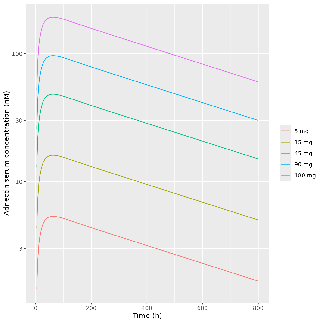
print(p2)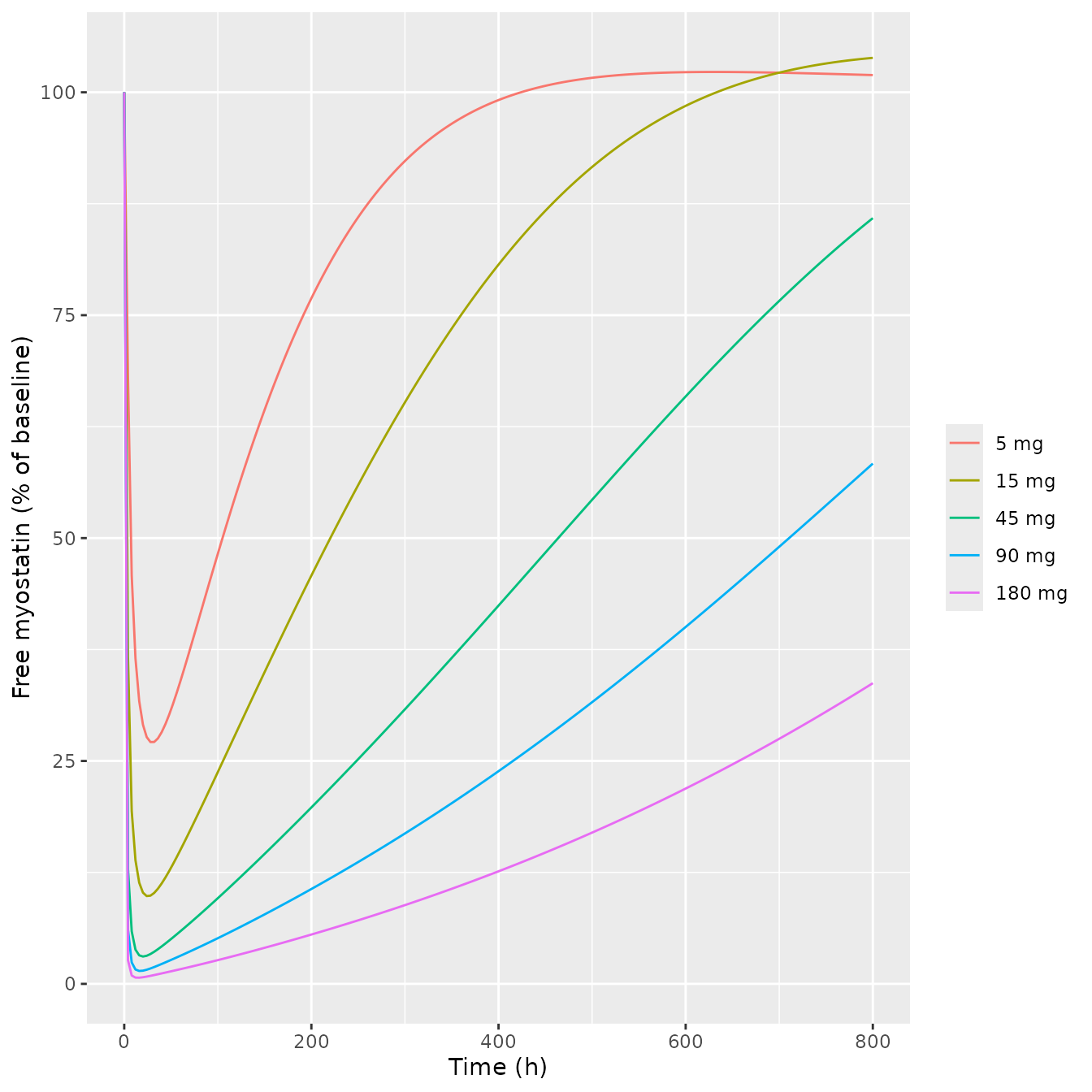
print(p3)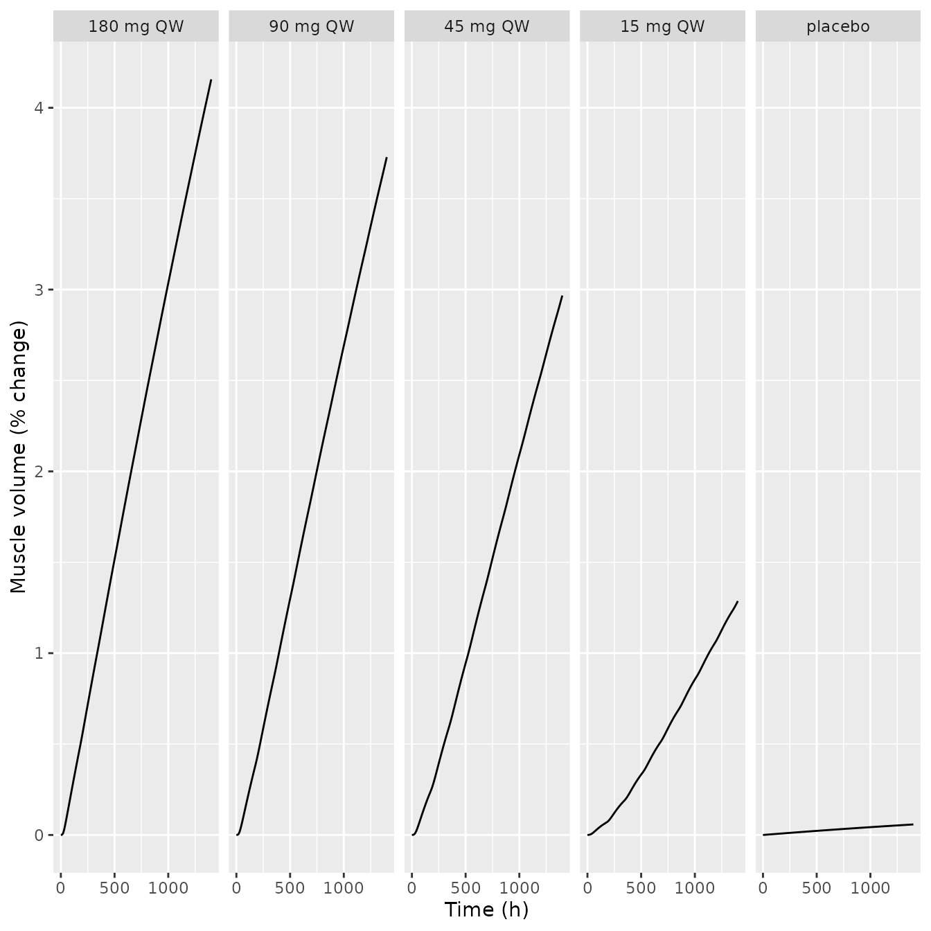
Replicates Figure 2 of Nguyen 2020 (single subcutaneous doses of 5-180 mg for PK and free myostatin; weekly doses for muscle volume). The simulated peaks (about 5 nM at 5 mg and 190 nM at 180 mg) and the dose-ordered suppression and recovery of free myostatin match the published panels. Muscle volume at 1300 h is compared below with the fitted curves, read off the lower panels of Figure 2 by the maintainers (approximate):
fig2_read <- data.frame(dose = paste(c(180, 90, 45, 15), "mg QW"), fig2 = c(4.2, 3.8, 3.0, 1.0))
adn_mus |>
  filter(time == 1300, dose != "placebo") |>
  transmute(dose = as.character(dose), sim = round(muscle_growth, 2)) |>
  inner_join(fig2_read, by = "dose") |>
  rename("Regimen" = dose, "Simulated (%)" = sim, "Figure 2 curve (%)" = fig2) |>
knitr::kable(caption = "Muscle-volume change at 1300 h, weekly adnectin.")| Regimen | Simulated (%) | Figure 2 curve (%) |
|---|---|---|
| 15 mg QW | 1.18 | 1.0 |
| 45 mg QW | 2.76 | 3.0 |
| 90 mg QW | 3.48 | 3.8 |
| 180 mg QW | 3.88 | 4.2 |
ACE-031 (Figure 3 and Table 3)
ace <- bind_rows(lapply(c(0.3, 1, 3), function(d) {
  solve_df(mods$ace031, et(amt = d * bw_human, cmt = "depot") |> et(seq(0, 2880, by = 4))) |>
    mutate(dose = paste(d, "mg/kg"))
}))
ggplot(filter(ace, time >= 1, time <= 1400), aes(time, Cc, colour = dose)) +
  geom_line() +
  scale_y_log10() +
  labs(x = "Time (h)", y = "ACE-031 serum concentration (ng/mL)", colour = NULL)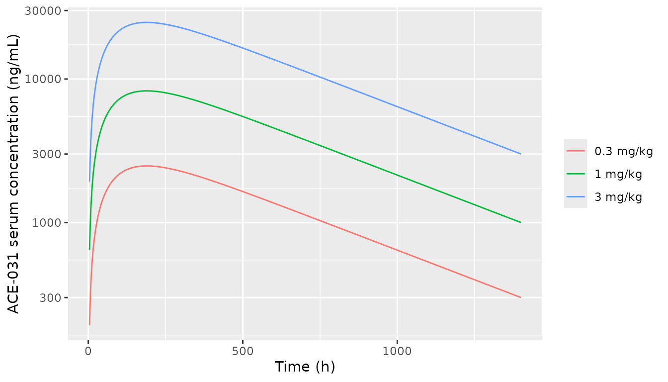
ggplot(filter(ace, time <= 1400), aes(time, fsh)) +
  geom_line() +
  facet_wrap(~dose) +
  labs(x = "Time (h)", y = "Plasma FSH (ng/mL)")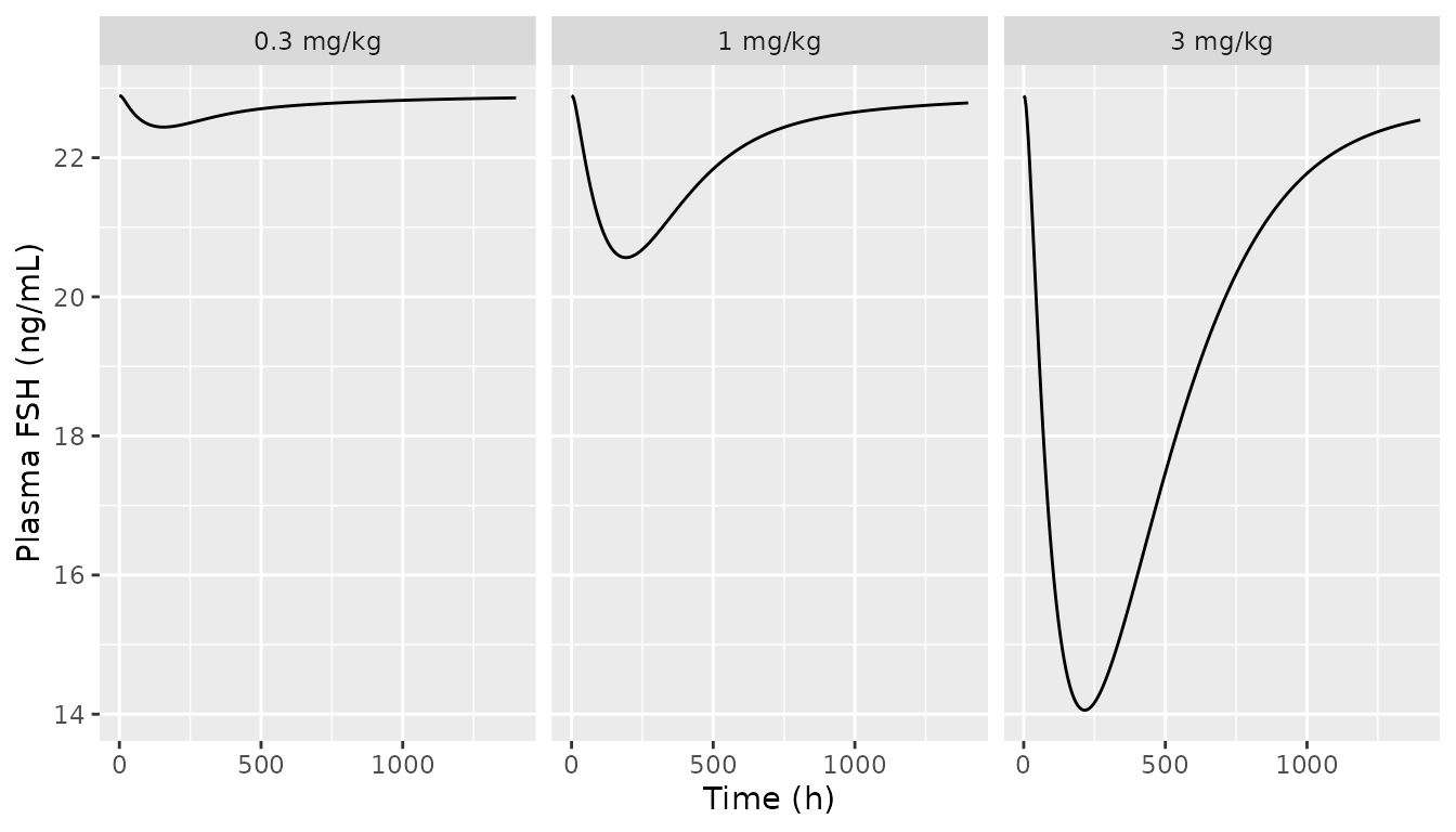
Replicates Figure 3 of Nguyen 2020 (single subcutaneous doses). The PK matches the published curves: Cmax of about 1900, 7400 and 24000 ng/mL at 0.3, 1 and 3 mg/kg. The model’s baseline FSH is 22.9 ng/mL, against about 24-25 ng/mL in the published panels.
ace_summary <- ace |>
  group_by(dose) |>
  summarise(
    mg_peak = max(muscle_growth),
    fsh_nadir_pct = 100 * (min(fsh) / first(fsh) - 1),
    .groups = "drop"
  )
knitr::kable(
  ace_summary |>
    mutate(across(where(is.numeric), \(x) round(x, 2))) |>
    rename("Dose" = dose, "Peak muscle-volume change (%)" = mg_peak, "FSH nadir (% change)" = fsh_nadir_pct),
  caption = "ACE-031 single subcutaneous dose: muscle volume and FSH."
)| Dose | Peak muscle-volume change (%) | FSH nadir (% change) |
|---|---|---|
| 0.3 mg/kg | 0.22 | -1.97 |
| 1 mg/kg | 1.44 | -10.17 |
| 3 mg/kg | 3.15 | -38.59 |
Table 3 reports simulated muscle-volume increases of 2.0% (1 mg/kg) and 3.14% (3 mg/kg) for ACE-031. The packaged model reproduces the 3 mg/kg value (3.15%). At 3 mg/kg the FSH nadir, -39%, is also close to the 43% decrease observed after a single 3 mg/kg dose. The 1 mg/kg value does not reproduce: the model gives 1.44%, 28% below the printed 2.0%. The same dose shows a shallower FSH dip than the 1 mg/kg panel of Figure 3 (-10% vs about -30%). The PK at 1 mg/kg matches Figure 3, and the gap is unchanged with the deposited code’s receptor rate constants (1.45%). It therefore looks like a feature of the authors’ 1 mg/kg simulation that cannot be recovered from the paper, not a transcription error in the model.
Domagrozumab (Table 3)
Table 3 gives a simulated increase of 5.64% for domagrozumab 10 mg/kg but does not state the regimen. The simulations below bracket plausible intravenous regimens:
dom_regimens <- list(
  "single dose" = et(amt = 10 * bw_human, cmt = "central"),
  "q4w x 3" = et(amt = 10 * bw_human, cmt = "central", ii = 672, addl = 2),
  "q2w x 6" = et(amt = 10 * bw_human, cmt = "central", ii = 336, addl = 5)
)
dom_tab <- bind_rows(lapply(names(dom_regimens), function(r) {
  s <- solve_df(mods$domagrozumab, dom_regimens[[r]] |> et(seq(0, 2880, by = 24)))
  data.frame(regimen = r, day85 = s$muscle_growth[s$time == 85 * 24], peak = max(s$muscle_growth))
}))
dom_tab |>
  mutate(across(where(is.numeric), \(x) round(x, 2))) |>
  rename("10 mg/kg IV regimen" = regimen, "Muscle change at day 85 (%)" = day85, "Peak within 120 days (%)" = peak) |>
knitr::kable(caption = "Domagrozumab 10 mg/kg: simulated muscle-volume change (Table 3 simulated 5.64%).")| 10 mg/kg IV regimen | Muscle change at day 85 (%) | Peak within 120 days (%) |
|---|---|---|
| single dose | 2.92 | 2.98 |
| q4w x 3 | 5.31 | 6.26 |
| q2w x 6 | 5.79 | 7.37 |
The published 5.64% lies between the single-dose value and the multiple-dose values, which is consistent. It cannot be checked more closely without the regimen.
Validation 3: FS-EEE-Fc in preclinical species (Figures S5-S6)
mouse_pk <- solve_df(mods$mouse, et(amt = 1 * 0.028, cmt = "central") |> et(c(0.083, seq(1, 168, by = 1)))) |>
  mutate(study = "mouse 1 mg/kg IV")
rat_pk <- bind_rows(lapply(c(0.1, 1, 10), function(d) {
  solve_df(mods$rat, et(amt = d * 0.28, cmt = "central") |> et(c(0.083, seq(1, 400, by = 1)))) |>
    mutate(study = paste("rat", d, "mg/kg IV"))
}))
monkey_pk <- bind_rows(
  lapply(c(0.3, 3, 30), function(d) {
    solve_df(mods$monkey, et(amt = d * 6.2, cmt = "central") |> et(c(0.083, seq(1, 1008, by = 1)))) |>
      mutate(study = paste("monkey", d, "mg/kg IV"))
  }),
  solve_df(mods$monkey, et(amt = 3 * 6.2, cmt = "depot") |> et(seq(0, 1008, by = 1))) |>
    mutate(study = "monkey 3 mg/kg SC")
)
ggplot(filter(bind_rows(mouse_pk, rat_pk, monkey_pk), time >= 1), aes(time, Cc, colour = study)) +
  geom_line() +
  scale_y_log10() +
  labs(x = "Time (h)", y = "Total FS-EEE-Fc in serum (ng/mL)", colour = NULL)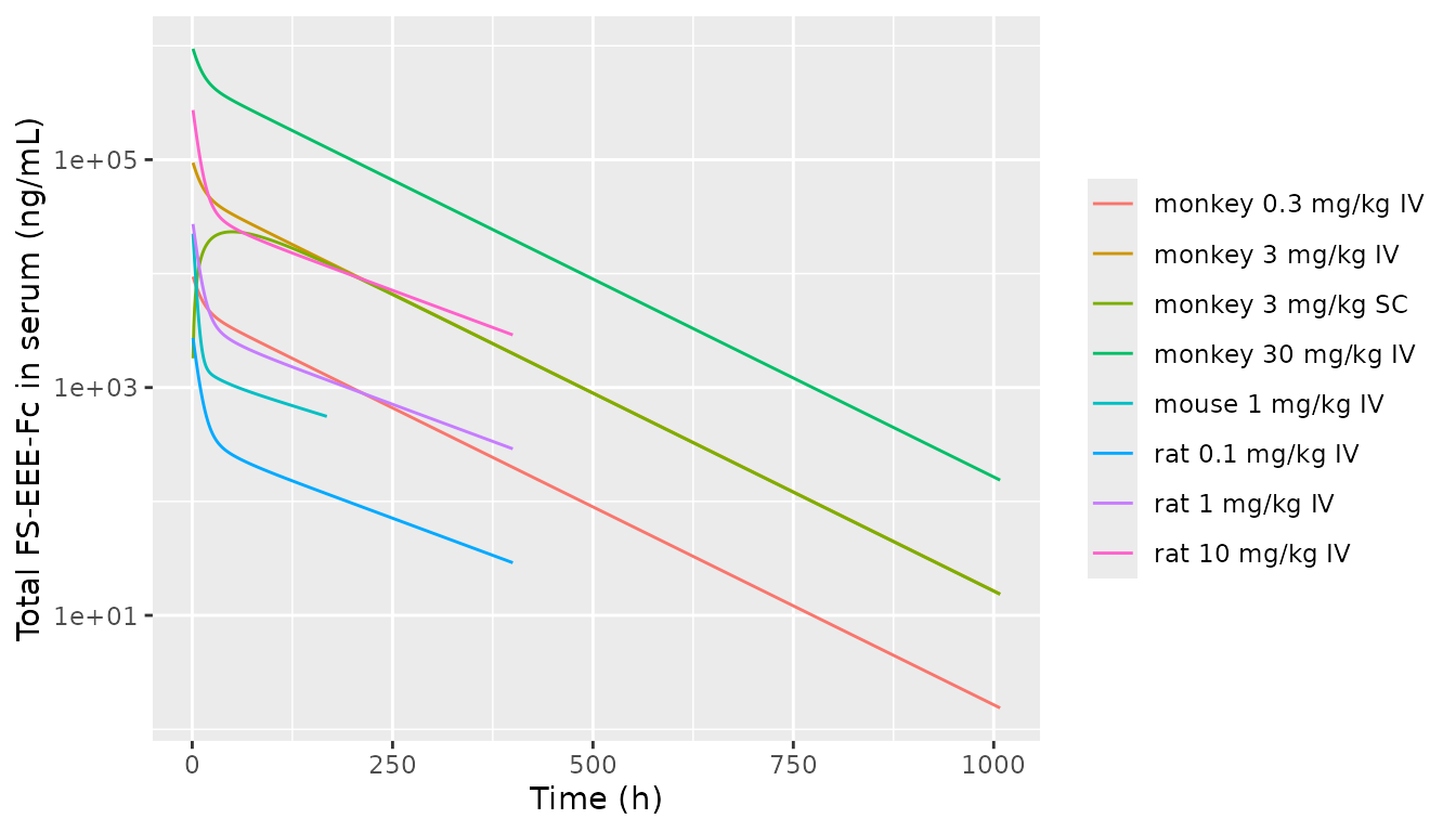
Replicates Figure S5 (mouse and monkey PK) and the unlabelled FS-EEE-Fc 0.1/1/10 mg/kg PK panel of the supplement. That panel’s initial concentrations (about 3e3, 3e4 and 3e5 ng/mL) identify it as the rat. Concentrations read off the published fitted lines by the maintainers (approximate) are compared below. This is where total drug and free drug separate: at 0.1 mg/kg the free drug at 400 h is less than half the total, and only the total matches the published line.
pk_read <- data.frame(
  study = c("mouse 1 mg/kg IV", "rat 0.1 mg/kg IV", "rat 1 mg/kg IV", "rat 10 mg/kg IV", "monkey 3 mg/kg IV", "monkey 30 mg/kg IV"),
  time = c(168, 400, 400, 400, 840, 1008),
  fig = c(500, 30, 300, 3000, 50, 120)
)
bind_rows(mouse_pk, rat_pk, monkey_pk) |>
  inner_join(pk_read, by = c("study", "time")) |>
  transmute(study, time, fig, Cc = signif(Cc, 3), Cfree = signif(Cfree, 3)) |>
  rename("Study" = study, "Time (h)" = time, "Published line (ng/mL)" = fig, "Simulated total, Cc" = Cc, "Simulated free, Cfree" = Cfree) |>
knitr::kable(caption = "FS-EEE-Fc preclinical PK, published fitted lines vs simulation.")| Study | Time (h) | Published line (ng/mL) | Simulated total, Cc | Simulated free, Cfree |
|---|---|---|---|---|
| mouse 1 mg/kg IV | 168 | 500 | 558 | 339.0 |
| rat 0.1 mg/kg IV | 400 | 30 | 29 | 11.2 |
| rat 1 mg/kg IV | 400 | 300 | 290 | 142.0 |
| rat 10 mg/kg IV | 400 | 3000 | 2900 | 2380.0 |
| monkey 3 mg/kg IV | 840 | 50 | 59 | 11.4 |
| monkey 30 mg/kg IV | 1008 | 120 | 154 | 30.0 |
mouse_mus <- bind_rows(lapply(c(0, 1, 3, 10, 50), function(d) {
  ev <- if (d > 0) et(amt = d * 0.028, cmt = "central", ii = 84, addl = 7) |> et(seq(0, 672, by = 6)) else et(seq(0, 672, by = 6))
  solve_df(mods$mouse, ev) |> mutate(dose = if (d > 0) paste(d, "mg/kg") else "vehicle")
}))
rat_fsh <- bind_rows(lapply(c(1, 3, 10), function(d) {
  solve_df(mods$rat, et(amt = d * 0.28, cmt = "central") |> et(seq(0, 336, by = 1))) |> mutate(dose = paste(d, "mg/kg"))
}))
ggplot(mouse_mus, aes(time / 24, muscle_growth, colour = dose)) +
  geom_line() +
  labs(x = "Time (day)", y = "Muscle mass (% change)", colour = "IV twice weekly")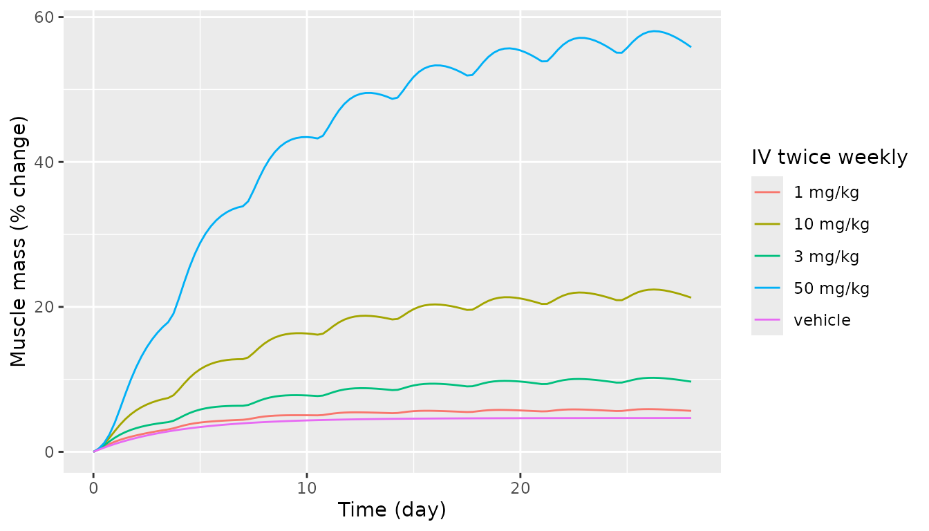
ggplot(rat_fsh, aes(time, fsh, colour = dose)) +
  geom_line() +
  labs(x = "Time (h)", y = "FSH (ng/mL)", colour = "Single IV dose")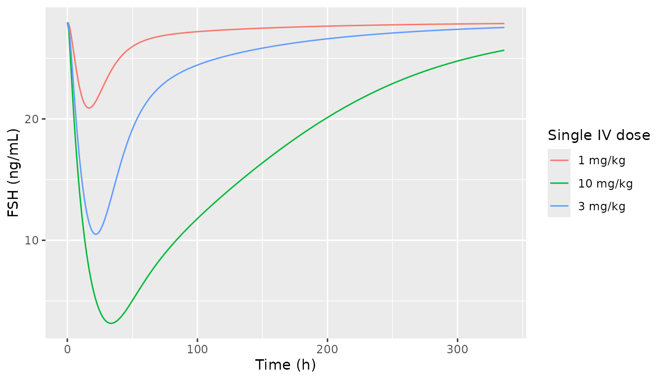
mouse_d28 <- mouse_mus |> filter(time == 672)
rat_nadir <- rat_fsh |> group_by(dose) |> summarise(nadir = min(fsh), t_nadir = time[which.min(fsh)], .groups = "drop")
knitr::kable(
  data.frame(
    dose = mouse_d28$dose, sim = round(mouse_d28$muscle_growth, 1),
    fig = c(NA, 6, 10, 19, 55)
  ) |> rename("Mouse dose (IV twice weekly)" = dose, "Day-28 muscle mass, sim (%)" = sim, "Figure S6A (%)" = fig),
  caption = "Mouse muscle mass at day 28 (Figure S6A read by the maintainers, approximate)."
)| Mouse dose (IV twice weekly) | Day-28 muscle mass, sim (%) | Figure S6A (%) |
|---|---|---|
| vehicle | 4.7 | NA |
| 1 mg/kg | 5.7 | 6 |
| 3 mg/kg | 9.7 | 10 |
| 10 mg/kg | 21.3 | 19 |
| 50 mg/kg | 55.8 | 55 |
knitr::kable(
  rat_nadir |>
    mutate(fig_nadir = c(21.5, 11, 3.5)[match(dose, c("1 mg/kg", "3 mg/kg", "10 mg/kg"))], nadir = round(nadir, 1)) |>
    rename("Rat dose (single IV)" = dose, "FSH nadir, sim (ng/mL)" = nadir, "Time of nadir, sim (h)" = t_nadir, "Figure S6B nadir (ng/mL)" = fig_nadir),
  caption = "Ovariectomised-rat FSH nadir (Figure S6B read by the maintainers, approximate)."
)| Rat dose (single IV) | FSH nadir, sim (ng/mL) | Time of nadir, sim (h) | Figure S6B nadir (ng/mL) |
|---|---|---|---|
| 1 mg/kg | 20.9 | 17 | 21.5 |
| 10 mg/kg | 3.2 | 34 | 3.5 |
| 3 mg/kg | 10.5 | 22 | 11.0 |
Replicates Figures S6A and S6B. The mouse muscle-mass curves reach about 6, 10, 21 and 56% at day 28 (published fitted curves about 6, 10, 19 and 55%). The rat FSH nadirs, about 21, 10.5 and 3 ng/mL at 17-34 h from a baseline of 28 ng/mL, match Figure S6B. The vehicle curve shows the drug-free drift of the indirect-response term in the mouse. Mouse baseline occupancy is 91%, so the term settles within days at about 4.7%. The published data likewise start near 3%.
Model applications to FS-EEE-Fc (Figure 4)
fs_dual <- bind_rows(
  solve_df(mods$fseeefc, et(amt = 3 * bw_human, cmt = "depot", ii = 168, addl = 5) |> et(seq(0, 2000, by = 4))) |>
    mutate(case = "Myostatin + activin inhibitor"),
  solve_df(mods$fseeefc, et(amt = 3 * bw_human, cmt = "depot", ii = 168, addl = 5) |> et(seq(0, 2000, by = 4)),
    params = c(koff_drug_act = 6e5)
  ) |>
    mutate(case = "Myostatin inhibitor")
)
ggplot(fs_dual, aes(time, ro_muscle, colour = case)) +
  geom_line() +
  labs(x = "Time (h)", y = "ActRIIB total RO in muscle (%)", colour = NULL)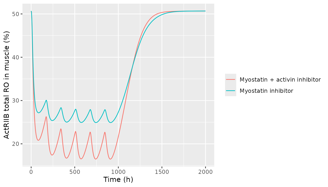
ro_trough <- fs_dual |>
  filter(time > 500, time < 1000) |>
  group_by(case) |>
  summarise(ro_min = min(ro_muscle), .groups = "drop")
knitr::kable(ro_trough |> mutate(ro_min = round(ro_min, 1)) |> rename("Case" = case, "Minimum muscle RO under dosing (%)" = ro_min))| Case | Minimum muscle RO under dosing (%) |
|---|---|
| Myostatin + activin inhibitor | 16.5 |
| Myostatin inhibitor | 24.9 |
Replicates the idea of Figure 4a (six weekly 3 mg/kg subcutaneous
doses; the published dose is not stated). Here the myostatin-only
molecule is the same model with activin binding switched off
(koff_drug_act set to the “arbitrary high” 6e5 1/h that
Table 2 uses for the myostatin-only compounds). Adding activin
neutralisation lowers the minimum muscle occupancy by about 8 percentage
points, against about 10 in the paper.
fs_doses <- c(1, 3, 5, 10, 30)
fs <- bind_rows(lapply(fs_doses, function(d) {
  solve_df(mods$fseeefc, et(amt = d * bw_human, cmt = "depot", ii = 168, addl = 25) |> et(seq(0, 180 * 24, by = 6))) |>
    mutate(dose = factor(paste(d, "mg/kg"), levels = paste(rev(fs_doses), "mg/kg")))
}))
ggplot(filter(fs, time >= 24), aes(time / 24, Cc, colour = dose)) +
  geom_line() +
  scale_y_log10(limits = c(1e3, 1e6)) +
  labs(x = "Time (day)", y = "Total drug in plasma (ng/mL)", colour = "Weekly SC")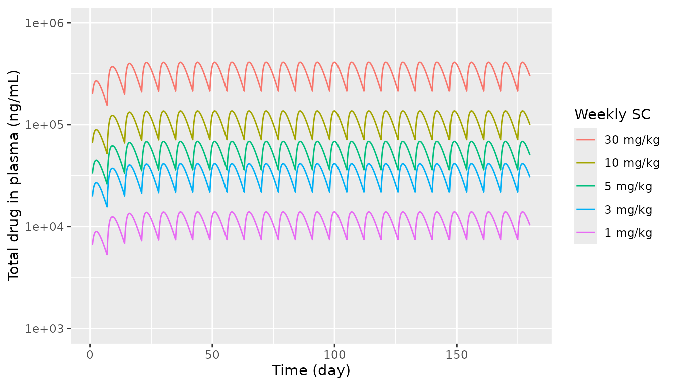
ggplot(fs, aes(time / 24, muscle_growth, colour = dose)) +
  geom_line() +
  geom_hline(yintercept = 7, linetype = "dashed") +
  labs(x = "Time (day)", y = "Muscle volume (% change)", colour = "Weekly SC")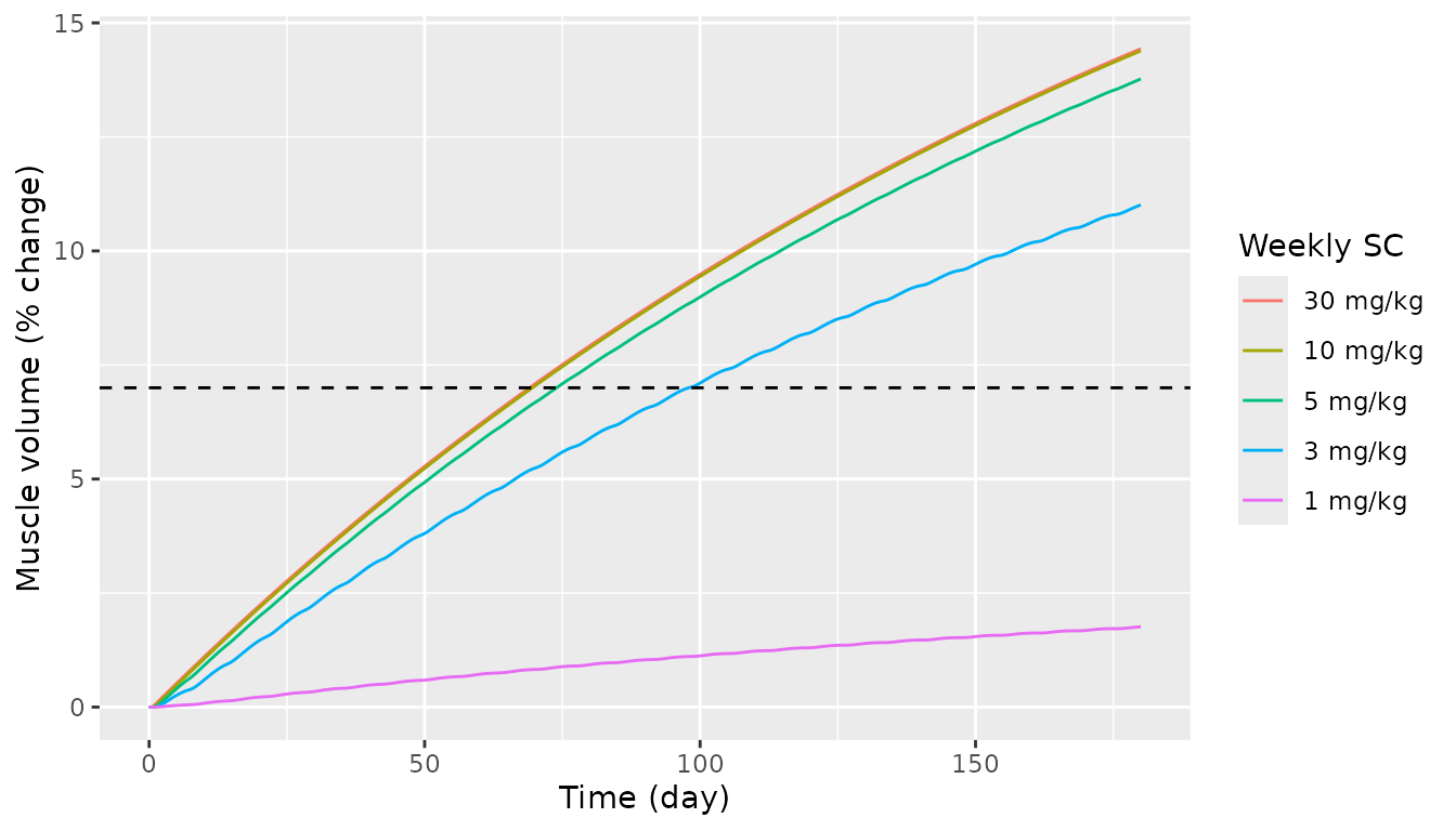
fs_120 <- fs |> filter(time == 120 * 24) |> select(dose, mg120 = muscle_growth)
fs_180 <- fs |> filter(time == 180 * 24) |> select(dose, mg180 = muscle_growth)
fs_tab <- inner_join(fs_120, fs_180, by = "dose") |> arrange(desc(dose))
knitr::kable(
  fs_tab |>
    mutate(fig4d_180 = c(1.3, 9.5, 13, 13.3, 13.5), across(where(is.numeric), \(x) round(x, 1))) |>
    rename("Weekly SC dose" = dose, "Day 120 (%)" = mg120, "Day 180 (%)" = mg180, "Figure 4d, day 180 (%)" = fig4d_180),
  caption = "FS-EEE-Fc muscle-volume projection (Figure 4d read by the maintainers, approximate)."
)| Weekly SC dose | Day 120 (%) | Day 180 (%) | Figure 4d, day 180 (%) |
|---|---|---|---|
| 1 mg/kg | 1.3 | 1.8 | 1.3 |
| 3 mg/kg | 8.2 | 11.0 | 9.5 |
| 5 mg/kg | 10.4 | 13.8 | 13.0 |
| 10 mg/kg | 10.9 | 14.4 | 13.3 |
| 30 mg/kg | 10.9 | 14.4 | 13.5 |
stopifnot(
  # 1 mg/kg weekly stays far below the 7% efficacy threshold ...
  fs_tab$mg180[fs_tab$dose == "1 mg/kg"] < 7,
  # ... and 3 mg/kg and above cross it within the 24-week horizon.
  all(fs_tab$mg180[fs_tab$dose != "1 mg/kg"] > 7)
)
Replicates Figures 4c and 4d of Nguyen 2020. The weekly profiles span the published 1e4-1e5+ ng/mL range and order by dose. The muscle-volume projection reproduces the paper’s conclusion: 1 mg/kg weekly is far short of the 7% efficacy threshold, 3 mg/kg crosses it before day 120 (8.2% at day 120), and 5 mg/kg and above approach the same plateau. The simulated day-180 values run about 0.5-1.5 percentage points above the curves read off Figure 4d. The deposited code’s parameter values do not close the gap (they raise the projection slightly; see the sensitivity section).
PKNCA: single-dose exposure of the human compounds
Nguyen 2020 reports no NCA parameters, so there is no published-vs-simulated NCA table. The block below records the typical-value single-dose exposure of each human model at a representative dose, grouped by compound.
nca_runs <- list(
  "FS-EEE-Fc 3 mg/kg SC" = list(mod = mods$fseeefc, ev = et(amt = 3 * bw_human, cmt = "depot"), dose = 3 * bw_human),
  "Adnectin 180 mg SC" = list(mod = mods$adnectin, ev = et(amt = 180, cmt = "depot"), dose = 180),
  "ACE-031 3 mg/kg SC" = list(mod = mods$ace031, ev = et(amt = 3 * bw_human, cmt = "depot"), dose = 3 * bw_human),
  "Domagrozumab 10 mg/kg IV" = list(mod = mods$domagrozumab, ev = et(amt = 10 * bw_human, cmt = "central"), dose = 10 * bw_human)
)
nca_conc <- bind_rows(lapply(names(nca_runs), function(k) {
  r <- nca_runs[[k]]
  solve_df(r$mod, r$ev |> et(c(0, 1, 2, 4, 8, 12, seq(24, 2016, by = 24)))) |>
    transmute(id = 1L, time, Cc = Cc / 1000, treatment = k)
})) |>
  filter(!is.na(Cc))
nca_dose <- data.frame(id = 1L, time = 0, treatment = names(nca_runs), amt = vapply(nca_runs, `[[`, numeric(1), "dose"))
conc_obj <- PKNCAconc(nca_conc, Cc ~ time | treatment + id, concu = "ug/mL", timeu = "h")
dose_obj <- PKNCAdose(nca_dose, amt ~ time | treatment + id, doseu = "mg")
intervals <- data.frame(start = 0, end = Inf, cmax = TRUE, tmax = TRUE, aucinf.obs = TRUE, half.life = TRUE)
nca_res <- pk.nca(PKNCAdata(conc_obj, dose_obj, intervals = intervals))
as.data.frame(nca_res) |>
  filter(PPTESTCD %in% c("cmax", "tmax", "aucinf.obs", "half.life")) |>
  select(treatment, PPTESTCD, PPORRES) |>
  mutate(PPORRES = signif(PPORRES, 3)) |>
  pivot_wider(names_from = PPTESTCD, values_from = PPORRES) |>
  rename("Treatment" = treatment, "Cmax (ug/mL)" = cmax, "Tmax (h)" = tmax, "AUC0-inf (h*ug/mL)" = aucinf.obs, "t1/2 (h)" = half.life) |>
knitr::kable(caption = "Typical-value single-dose NCA of total drug.")| Treatment | Cmax (ug/mL) | Tmax (h) | t1/2 (h) | AUC0-inf (h*ug/mL) |
|---|---|---|---|---|
| ACE-031 3 mg/kg SC | 24.8 | 192 | 367 | 18800 |
| Adnectin 180 mg SC | 14.6 | 72 | 433 | 10000 |
| Domagrozumab 10 mg/kg IV | 227.0 | 0 | 493 | 153000 |
| FS-EEE-Fc 3 mg/kg SC | 26.5 | 72 | 109 | 5650 |
Sensitivity to the table-versus-code parameter differences
The packaged models use the printed tables. Two groups of values differ from the deposited human FS-EEE-Fc code. Changing them has little effect on the projection:
code_values <- c(
  kon_myo_actriib = 0.6, koff_myo_actriib = 0.6 * 0.0935,
  kon_act_actriib = 0.6, koff_act_actriib = 0.6 * 0.0357,
  kdeg_md = 0.008, kdeg_ad = 0.008
)
ev_code <- et(amt = 3 * bw_human, cmt = "depot", ii = 168, addl = 24) |> et(seq(0, 25 * 168, by = 24))
s_tab <- solve_df(mods$fseeefc, ev_code)
s_code <- solve_df(mods$fseeefc, ev_code, params = code_values)
knitr::kable(data.frame(
  quantity = c("Total drug at the last dose (ng/mL)", "Muscle-volume change at the last dose (%)"),
  tables = signif(c(tail(s_tab$Cc, 1), tail(s_tab$muscle_growth, 1)), 4),
  code = signif(c(tail(s_code$Cc, 1), tail(s_code$muscle_growth, 1)), 4)
) |> rename("Quantity (3 mg/kg weekly x 25)" = quantity, "Published tables" = tables, "Deposited-code values" = code))| Quantity (3 mg/kg weekly x 25) | Published tables | Deposited-code values |
|---|---|---|
| Total drug at the last dose (ng/mL) | 21650.00 | 21190.00 |
| Muscle-volume change at the last dose (%) | 10.79 | 10.89 |
Assumptions and deviations
-
FSH equation. The Supplementary Methods print
dFSH/dt = Vmax_FSH * (1 - RO^h / (RO^h + RO50^h)) - kdeg_FSH * FSH. The deposited code usesVmax_FSH * RO^h / (RO^h + RO50^h), so FSH production rises with pituitary occupancy. Only the code’s form makes FSH fall when an activin trap lowers pituitary occupancy, which is the 43% ACE-031 decrease the text describes and the direction of Figures 3 and S6B. The printed form would raise FSH. The packaged models use the code’s form. Table 2 labels RO50_FSH “%RO leads to 50% FSH decrease”, which is consistent with this. - Receptor rate constants. Table 1 (and Table S3) give kon/koff = 1.328 1/(nM h) / 0.124 1/h for myostatin-ActRIIB and 14.90 / 0.533 for activin-ActRIIB. The deposited code uses kon = 0.6 with the same dissociation constants (93.5 and 35.7 pM). The packaged models use the tables. The steady state depends only on the dissociation constants and is identical either way. The effect on the projection is shown above.
- Complex degradation for FS-EEE-Fc. Table 2 prints k_deg_MD = k_deg_AD = 0.006 1/h (“assumed ~ k_deg_drug”), while k_deg_drug = 0.008 1/h and the deposited code clears complexes at k_deg_drug. The packaged human FS-EEE-Fc model uses the printed 0.006. For every other compound and species the two values are equal.
- Extra digits from the code. Where the deposited code carries more digits than Table 1 (lymph flows, ligand synthesis, cleavage and degradation rates), the code value is used. Every such value rounds to the printed one.
- Synthesis-rate units. Table 1 prints the ligand synthesis rates in 1/hour, but the code adds them to the amount balance directly (nmol/h). The labels use nmol/h.
-
Drug-free run-in replaced by an analytic steady
state. See Implementation notes. The authors’ 1000 h run-in and
the analytic start are the same fixed point of the ODEs, and the check
above shows no drift over 2000 h. The deposited code’s mass-balance
bookkeeping states and its
Percent_Free_Myooutput (normalised by a hard-codedDummy1 = 0.01945) are not reproduced. They do not feed back on any other state. Free myostatin is available asmyo_free_plasma. -
Muscle-growth start. As in the code,
muscle_growthstarts at 0 at the first dose and includes a slow drug-free drift toward the baseline-occupancy steady state: about 0.24% over years in humans, but about 4.7% within days in mice. -
Domagrozumab route. Table 2 prints F = 0.75 but no
ka for domagrozumab, so only intravenous dosing into
centralis encoded. The mouse and rat also have no ka or F in Table S4 and are IV-only. - Preclinical assumptions. Table S3 does not repeat the molecular weights of the ligands, so the Table 1 values are used. The ActRIIB concentration (0.138 nM) is printed once for all species and applied to each. The degradation rates and reflection coefficients apply to every tissue, per the table footnotes. Only the mouse carries a muscle sub-model and only the rat an FSH sub-model, because only those were parameterised (Table S4).
- Table 3, ACE-031 1 mg/kg. Not reproduced (1.44% vs 2.0%); see Validation 2.
- Values read off figures. The published comparison values in the tables above (Figures 2, 4d, S5, S6) were read off the figures by the maintainers. They are approximate and are shown for orientation only. None of them enters a model parameter.