Zolpidem CNS pharmacodynamics (Kim 2026)

Model and source

Citation: Kim HC, Sunwoo J, Yoon S, Jang I-J, Chung J-Y. Population Pharmacokinetic-Pharmacodynamic Analysis of Zolpidem in Healthy Volunteers: Covariate Contributions to Variability in CNS Responses. CPT Pharmacometrics Syst Pharmacol. 2026;15:e70208. doi:10.1002/psp4.70208
Article: https://doi.org/10.1002/psp4.70208
Supplementary Data S1-S4: the four deposited NONMEM control streams

Kim 2026 gave 30 healthy Korean volunteers a single 10 mg oral dose of immediate-release zolpidem and measured three central-nervous-system responses alongside plasma concentration: the digit symbol substitution test (DSST, cognitive), choice reaction time (CRT, psychomotor) and a self-rated sedation visual analog scale (VAS, subjective). The question behind the paper is regulatory: the U.S. FDA halved the recommended starting dose for women in 2013, while the EMA and the Korean MFDS did not, and the authors ask whether the apparent sex difference is really sex or is instead mediated by body weight, albumin, age and baseline CNS performance.

Each PD endpoint was fitted sequentially to the same final PK model, as four separate NONMEM runs. That structure is reproduced here as four model files rather than one, because the PK parameters are estimated in the first run and fixed in the other three – a distinction that a single merged file could not express:

Model file	Deposited control stream	What is estimated
`Kim_2026_zolpidem`	Data S1	The PK parameters themselves
`Kim_2026_zolpidem_dsst`	Data S2	DSST response + learning effect; PK fixed
`Kim_2026_zolpidem_crt`	Data S3	CRT response; PK fixed
`Kim_2026_zolpidem_vas`	Data S4	VAS response + spline baseline; PK fixed

The three PD control streams each declare a COMP(EFFECT) compartment, but none of them writes a differential equation for it or ever references it: an effect-compartment model was tested and rejected for VAS (dOFV = -2.524, Results 3.2.4), and the declaration is a leftover. All three final models are direct-response, so no effect compartment is reproduced here.

A note on time. Methods 2.1 redefines the first Day -1 assessment (-23 h) as t = 1 h, which places dosing at t = 24 h. Two parts of the model depend on that absolute clock – the DSST learning term, and the VAS baseline spline – so every event table below doses at 24 h, not at 0 h.

Population

Species: human
Subjects: 30 (50% female)
Age: 20-44 years (median 29.5 years)
Weight: 50.0-83.0 kg (median 60.05 kg)
Disease state: healthy volunteers
Dose: single oral 10 mg immediate-release zolpidem
Region: Korea

Kim 2026 Table 1 gives baseline characteristics as median (min to max), both overall and by sex. Weight, albumin, ALT, AST, total bilirubin and serum creatinine all differed significantly between males and females, which is exactly the collinearity that motivates the paper.

Kim 2026 Table 1 (subset): baseline characteristics, median (min to max).
Variable	Total	Male	Female
Age (years)	29.5 (20 to 44)	31 (20 to 42)	27 (24 to 44)
Weight (kg)	60.05 (50.0 to 83.0)	75.4 (55.1 to 83.0)	54.9 (50.0 to 61.1)
Albumin (g/dL)	4.4 (3.9 to 5.0)	4.5 (4.1 to 5.0)	4.2 (3.9 to 4.8)
DSST at 1 h Day -1 (score)	72.5 (46 to 104)	63 (46 to 83)	74 (60 to 104)
CRT at 1 h Day -1 (msec)	438.5 (372 to 709)	438 (402 to 709)	453 (372 to 521)
VAS at 1 h Day -1 (mm)	30.5 (0 to 97)	24 (0 to 97)	48 (0 to 72)

Source trace

Every value in the four model files is traceable to Kim 2026 Table 2 or Table 3 and, independently, to the corresponding $THETA / $OMEGA entry of the deposited control stream. The two sources agree on every parameter except one, noted below.

Source trace for the model equations and parameters.
Quantity	Model parameter	Source location
Transit absorption input	`transit(nn, mtt, fdepot)`	Data S1 `$DES` (Savic closed form); Figure 1
One-compartment disposition	`d/dt(central)`	Data S1 `$DES`; Results 3.2.1
Ka 11.7 1/h	`lka`	Table 2; Data S1 `$THETA(3)`
CL/F 18.0 L/h	`lcl`	Table 2; Data S1 `$THETA(1)`
Vc/F 64.0 L	`lvc`	Table 2; Data S1 `$THETA(2)`
MTT 0.25 h	`lmtt`	Table 2; Data S1 `$THETA(4)`
NN 19.4	`lnn`	Table 2; Data S1 `$THETA(5)`
BIO 1 (fixed)	`lfdepot`	Table 2; Data S1 `$THETA(6)` FIX
PK proportional error 18.9%	`propSd`	Table 2; Data S1 `$THETA(7)`
DSST: IC50 205 ug/L	`lic50`	Table 3 DSST block; Data S2 `$THETA(9)`
DSST: HILL 2.54	`lhill`	Table 3 DSST block; Data S2 `$THETA(10)`
DSST: BASE 68.2 score	`lrbase`	Table 3 DSST block; Data S2 `$THETA(11)`
DSST: MAXlearn 14.4 score	`lemax_learn`	Table 3 DSST block; Data S2 `$THETA(12)`
DSST: LRPAR 4.3 h	`lt50_learn`	Table 3 DSST block; Data S2 `$THETA(13)`
DSST: weight on IC50, -1.57	`e_wt_ic50`	Table 3 row; Data S2 `$THETA(18)` (not footnote a – see Errata)
DSST: albumin on IC50, 0.541	`e_alb_ic50`	Table 3 row and footnote a; Data S2 `$THETA(17)`
DSST: age on BASE, -0.0143	`e_age_rbase`	Table 3 row and footnote b; Data S2 `$THETA(16)`
CRT: EC50 282 ug/L	`lec50`	Table 3 CRT block; Data S3 `$THETA(9)`
CRT: HILL 6	`lhill`	Table 3 CRT block; Data S3 `$THETA(12)`
CRT: BASE 437 msec	`lrbase`	Table 3 CRT block; Data S3 `$THETA(10)`
CRT: MAXdrug 5.6 (fixed)	`lemax`	Table 3 CRT block; Data S3 `$THETA(11)` FIX; Results 3.2.3
CRT: weight on EC50, -0.0193	`e_wt_ec50`	Table 3 row and footnote c; Data S3 `$THETA(18)`
CRT: albumin on EC50, 3.89	`e_alb_ec50`	Table 3 row and footnote c; Data S3 `$THETA(16)`
CRT: CRTB1 on EC50, -1.28	`e_crt_bl_ec50`	Table 3 row and footnote c; Data S3 `$THETA(17)`
CRT: albumin on HILL, -5.26	`e_alb_hill`	Table 3 row and footnote d; Data S3 `$THETA(19)`
CRT: CRTB1 on HILL, 0.00637	`e_crt_bl_hill`	Table 3 row and footnote d; Data S3 `$THETA(20)`
CRT: age on BASE, 0.0112	`e_age_rbase`	Table 3 row and footnote e; Data S3 `$THETA(15)`
VAS: EC50 146 ug/L	`lec50`	Table 3 VAS block; Data S4 `$THETA(9)`
VAS: HILL 1.92	`lhill`	Table 3 VAS block; Data S4 `$THETA(10)`
VAS: knots H1-H4	`logitrbase_t1`..`_t4`	Table 3 VAS block and Results 3.2.4; Data S4 `$THETA(11)`-`$THETA(14)`
VAS: logit transform of knots	`expit(logitrbase_ti + eta)`	Methods 2.3; Data S4 `$PK`
VAS: piecewise-linear spline	`vasbase`	Results 3.2.4 displayed equations; Data S4 `$ERROR`
VAS: headroom-bounded drug effect	`(100 - vasbase) * ...`	Results 3.2.4; Data S4 `$ERROR`

Reconciling the reported %CV against the encoded variances

Kim 2026 reports most inter-individual variabilities as %CV, with the note under Table 3 giving the transform used. The control-stream $OMEGA entries are variances. This block checks every reported %CV against the variance actually encoded in the model files – an enumerating check, so a mis-transcribed omega fails here rather than passing silently.

omega_of <- function(ui, eta) {
  df <- ui$iniDf
  df$est[!is.na(df$neta1) & df$neta1 == df$neta2 & df$name == eta]
}
pct_cv <- function(omega2) 100 * sqrt(exp(omega2) - 1)

cv_chk <- tibble::tribble(
  ~Model,  ~Parameter,   ~eta,           ~ui,      ~reported_cv,
  "PK",    "Ka",         "etalka",       "pk",     330.8,
  "PK",    "MTT",        "etalmtt",      "pk",      37.7,
  "PK",    "CL/F",       "etalcl",       "pk",      24.1,
  "PK",    "BIO",        "etalfdepot",   "pk",      25.9,
  "DSST",  "IC50",       "etalic50",     "dsst",    22.3,
  "DSST",  "BASE",       "etalrbase",    "dsst",    13.1,
  "CRT",   "EC50",       "etalec50",     "crt",     21.1,
  "CRT",   "BASE",       "etalrbase",    "crt",      9.4,
  "VAS",   "EC50",       "etalec50",     "vas",     53.9
) |>
  rowwise() |>
  mutate(
    omega2      = omega_of(get(paste0("ui_", ui)), eta),
    computed_cv = pct_cv(omega2)
  ) |>
  ungroup() |>
  mutate(abs_diff = abs(computed_cv - reported_cv))

# Every reported %CV is printed to 3 significant figures, so agreement must be
# within half a unit in the last printed place.
stopifnot(all(cv_chk$abs_diff < 0.05))

cv_chk |>
  select(Model, Parameter, omega2, computed_cv, reported_cv) |>
  mutate(across(c(omega2, computed_cv), ~ signif(.x, 4))) |>
  rename(
    "Encoded variance" = omega2,
    "%CV computed"     = computed_cv,
    "%CV reported"     = reported_cv
  ) |>
  knitr::kable(caption = "Every %CV in Kim 2026 Tables 2 and 3 reproduces from the encoded variance via 100 * sqrt(exp(omega^2) - 1).")

Every %CV in Kim 2026 Tables 2 and 3 reproduces from the encoded variance via 100 * sqrt(exp(omega^2) - 1).
Model	Parameter	Encoded variance	%CV computed	%CV reported
PK	Ka	2.48000	330.800	330.8
PK	MTT	0.13300	37.720	37.7
PK	CL/F	0.05650	24.110	24.1
PK	BIO	0.06470	25.850	25.9
DSST	IC50	0.04840	22.270	22.3
DSST	BASE	0.01710	13.130	13.1
CRT	EC50	0.04360	21.110	21.1
CRT	BASE	0.00871	9.353	9.4
VAS	EC50	0.25500	53.890	53.9

The four VAS baseline knots are the exception the paper flags: Table 3 footnote f states their IIV is “expressed as omega^2 instead of %CV”, so those four are read straight off the table with no transform.

vas_knot_omegas <- vapply(
  paste0("etalogitrbase_t", 1:4), omega_of, numeric(1), ui = ui_vas
)
# Table 3: 1.03, 0.653, 1.7, 0.699. The control stream gives 1.69 for the third,
# which is the unrounded value behind the table's 1.7.
stopifnot(all(abs(vas_knot_omegas - c(1.03, 0.653, 1.69, 0.699)) < 1e-12))
vas_knot_omegas
#> etalogitrbase_t1 etalogitrbase_t2 etalogitrbase_t3 etalogitrbase_t4 
#>            1.030            0.653            1.690            0.699

Virtual cohort

The cohort is rebuilt to Kim 2026 Table 1: 15 males and 15 females, with the sex-specific medians and ranges reproduced for the covariates the models actually use. Weight, albumin, age and baseline CRT are drawn from truncated normals calibrated so that the simulated median lands on the published median and the draw stays inside the published min-max. That distributional choice is an assumption – Table 1 reports only medians and ranges, not shapes.

Note that ALB is carried in the canonical register unit g/L, while Kim 2026 reports g/dL; the model files apply the register-mandated inline conversion, so the cohort below stores 44 g/L where the paper prints 4.4 g/dL.

set.seed(20260901)

rtrunc_median <- function(n, med, lo, hi) {
  # SD chosen so the published min-max spans roughly +/- 2 SD.
  x <- stats::rnorm(n, mean = med, sd = (hi - lo) / 4)
  pmin(pmax(x, lo), hi)
}

n_per_sex <- 15
cohort <- bind_rows(
  tibble::tibble(
    SEXF   = 0,
    WT     = rtrunc_median(n_per_sex, 75.4, 55.1, 83.0),
    ALB    = rtrunc_median(n_per_sex,  4.5,  4.1,  5.0) * 10, # g/dL -> canonical g/L
    AGE    = rtrunc_median(n_per_sex, 31,   20,   42),
    CRT_BL = rtrunc_median(n_per_sex, 438,  402,  709)
  ),
  tibble::tibble(
    SEXF   = 1,
    WT     = rtrunc_median(n_per_sex, 54.9, 50.0, 61.1),
    ALB    = rtrunc_median(n_per_sex,  4.2,  3.9,  4.8) * 10,
    AGE    = rtrunc_median(n_per_sex, 27,   24,   44),
    CRT_BL = rtrunc_median(n_per_sex, 453,  372,  521)
  )
) |>
  mutate(id = row_number(), sex = ifelse(SEXF == 1, "Female", "Male"))

cohort |>
  group_by(sex) |>
  summarise(
    n = n(),
    `Weight (kg)`      = sprintf("%.1f (%.1f-%.1f)", median(WT), min(WT), max(WT)),
    `Albumin (g/dL)`   = sprintf("%.2f (%.2f-%.2f)", median(ALB) / 10, min(ALB) / 10, max(ALB) / 10),
    `Age (years)`      = sprintf("%.0f (%.0f-%.0f)", median(AGE), min(AGE), max(AGE)),
    `CRT_BL (msec)`    = sprintf("%.0f (%.0f-%.0f)", median(CRT_BL), min(CRT_BL), max(CRT_BL)),
    .groups = "drop"
  ) |>
  rename(Sex = sex) |>
  knitr::kable(caption = "Simulated cohort, median (min-max), to be read against Kim 2026 Table 1.")

Simulated cohort, median (min-max), to be read against Kim 2026 Table 1.
Sex	n	Weight (kg)	Albumin (g/dL)	Age (years)	CRT_BL (msec)
Female	15	54.5 (50.2-58.1)	4.07 (3.90-4.44)	26 (24-33)	452 (372-509)
Male	15	75.2 (61.3-82.9)	4.54 (4.19-5.00)	33 (23-42)	447 (402-562)

Pharmacokinetics

Simulation

The PK model carries no absolute-time term, so the PK simulation doses at t = 0 and observes over the paper’s Day 1 sampling window (0-12 h). The PD simulations further down dose at t = 24 h, as the PD models require.

pk_grid <- sort(unique(c(seq(0, 12, by = 0.05),
                         c(0, 0.25, 0.5, 0.75, 1, 1.5, 2, 3, 4, 6, 8, 12))))

pk_events <- bind_rows(
  cohort |> transmute(id, time = 0, cmt = "depot", amt = 10, evid = 1L),
  tidyr::expand_grid(id = cohort$id, time = pk_grid) |>
    mutate(cmt = "central", amt = 0, evid = 0L)
) |>
  left_join(cohort |> select(id, WT, ALB, AGE, CRT_BL, SEXF, sex), by = "id") |>
  arrange(id, time, desc(evid)) |>
  as.data.frame()

rxode2::rxSetSeed(20260901)
pk_sim <- rxode2::rxSolve(ui_pk, pk_events, returnType = "data.frame") |>
  left_join(cohort |> select(id, sex), by = "id")

# rxode2's transit() has been observed to evaluate silently to zero through an
# rxUi handle on some builds. Assert that it did not, so this vignette can never
# ship an all-zero profile that merely looks like a flat plot.
stopifnot(max(pk_sim$Cc) > 1)

# Typical-value profile (all etas zeroed) at the cohort-median covariates.
typ_events <- data.frame(
  id = 1L,
  time = c(0, pk_grid),
  cmt = c("depot", rep("central", length(pk_grid))),
  amt = c(10, rep(0, length(pk_grid))),
  evid = c(1L, rep(0L, length(pk_grid)))
)
pk_typ <- rxode2::rxSolve(rxode2::zeroRe(ui_pk), typ_events, returnType = "data.frame")
#> ℹ omega/sigma items treated as zero: 'etalka', 'etalcl', 'etalmtt', 'etalfdepot'

Figure: plasma zolpidem concentration-time profile

Replicates the observation window of Kim 2026 Figure 2A (prediction-corrected VPC for plasma zolpidem) and Figure S2A.

# rxSolve returns one row per observation record, so no dose rows to filter out
# (and no `evid` column in the output).
pk_band <- pk_sim |>
  group_by(time) |>
  summarise(
    lo  = quantile(Cc, 0.05),
    mid = median(Cc),
    hi  = quantile(Cc, 0.95),
    .groups = "drop"
  )

ggplot(pk_band, aes(time)) +
  geom_ribbon(aes(ymin = lo, ymax = hi), alpha = 0.2, fill = "steelblue") +
  geom_line(aes(y = mid), colour = "steelblue", linewidth = 1) +
  geom_line(data = pk_typ, aes(time, Cc), linetype = "dashed") +
  labs(x = "Time after dose (h)", y = "Plasma zolpidem (ug/L)") +
  theme_bw()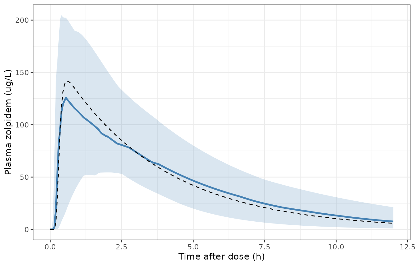

Simulated plasma zolpidem concentrations after a single 10 mg oral dose. Ribbon = 5th-95th percentile of the simulated cohort, solid line = median, dashed line = typical-value profile. Replicates the layout of Kim 2026 Figure 2A.

PKNCA validation

nca_conc <- pk_sim |>
  filter(!is.na(Cc)) |>
  transmute(id, time, Cc, treatment = "Zolpidem 10 mg single oral dose")

nca_dose <- pk_events |>
  filter(evid == 1) |>
  transmute(id, time, amt, treatment = "Zolpidem 10 mg single oral dose")

conc_obj <- PKNCA::PKNCAconc(nca_conc, Cc ~ time | treatment + id,
                             concu = "ug/L", timeu = "h")
dose_obj <- PKNCA::PKNCAdose(nca_dose, amt ~ time | treatment + id,
                             doseu = "mg")

intervals <- data.frame(
  start       = 0,
  end         = Inf,
  cmax        = TRUE,
  tmax        = TRUE,
  auclast     = TRUE,
  aucinf.obs  = TRUE,
  half.life   = TRUE,
  lambda.z    = TRUE
)

nca_res <- PKNCA::pk.nca(PKNCA::PKNCAdata(conc_obj, dose_obj, intervals = intervals))
nca_ind <- as.data.frame(nca_res)

Structural gate: AUC0-inf must equal Dose x F / CL, per subject

This is a self-consistency check rather than a comparison against a published number, and the two sides use the same drawn parameters, so a tight bound is the right one: the only difference is numerical (integration tolerance plus PKNCA’s terminal extrapolation from the 12 h profile). If the transit chain failed to deliver the whole dose, or the concentration scaling were wrong, this fails immediately.

auc_chk <- nca_ind |>
  filter(PPTESTCD == "aucinf.obs") |>
  transmute(id = as.integer(as.character(id)), aucinf = PPORRES) |>
  left_join(
    pk_sim |> group_by(id) |> summarise(cl = first(cl), fdepot = first(fdepot), .groups = "drop"),
    by = "id"
  ) |>
  mutate(
    auc_closed_form = 10 * fdepot / cl * 1000, # mg / (L/h) -> ug*h/L
    pct_diff = 100 * (aucinf - auc_closed_form) / auc_closed_form
  )

stopifnot(
  abs(median(auc_chk$pct_diff)) < 1,
  quantile(abs(auc_chk$pct_diff), 0.9) < 2
)

sprintf("AUC0-inf vs Dose*F/CL: median %.3f%%, 90th pctile |diff| %.3f%%",
        median(auc_chk$pct_diff), quantile(abs(auc_chk$pct_diff), 0.9))
#> [1] "AUC0-inf vs Dose*F/CL: median -0.001%, 90th pctile |diff| 0.133%"

Comparison against the published non-compartmental analysis

Kim 2026 does not tabulate its own NCA; the Introduction quotes the NCA of the source clinical study (reference 11, the same 30 subjects and the same 10 mg dose) for T_max and half-life, and those are the published values compared against here.

nca_simulated <- nca_ind |>
  filter(PPTESTCD %in% c("cmax", "tmax", "half.life", "aucinf.obs")) |>
  group_by(PPTESTCD) |>
  summarise(PPORRES = median(PPORRES), .groups = "drop") |>
  as.data.frame()

# Tmax reference is the midpoint of the published 0.5-0.75 h median range and
# half-life the midpoint of the published 2.9-3.1 h mean range, both quoted in
# Kim 2026 Introduction from the source clinical study (reference 11). Cmax and
# AUC0-inf were not reported there, so only the two published parameters can be
# compared.
nca_reference <- data.frame(
  PPTESTCD = c("tmax", "half.life"),
  PPORRES  = c(0.625, 3.0)
)

nlmixr2lib::ncaComparisonTable(
  simulated = nca_simulated,
  reference = nca_reference,
  units = c(cmax = "ug/L", tmax = "h", half.life = "h", aucinf.obs = "ug*h/L")
) |>
  knitr::kable(
    caption = paste(
      "Simulated median NCA parameters against the published values.",
      "Tmax reference is the midpoint of the reported 0.5-0.75 h median range;",
      "half-life reference is the midpoint of the reported 2.9-3.1 h mean range",
      "(Kim 2026 Introduction, citing the source clinical study)."
    )
  )

Simulated median NCA parameters against the published values. Tmax reference is the midpoint of the reported 0.5-0.75 h median range; half-life reference is the midpoint of the reported 2.9-3.1 h mean range (Kim 2026 Introduction, citing the source clinical study).
NCA parameter	Reference	Simulated	% diff
Tmax (h)	0.625	0.525	-16.0%
t½ (h)	3	2.61	-12.9%

For completeness, the simulated median C_max and AUC_0-inf, neither of which the paper reports:

Simulated median exposure metrics not reported by Kim 2026.
Parameter	Simulated
AUC0-inf (ug*h/L)	574.5
Cmax (ug/L)	132.1

The simulated median T_max falls inside the published 0.5-0.75 h window. The simulated half-life is shorter than the published NCA mean: the model’s disposition half-life is fixed by ln(2) x V_c/F / (CL/F) = ln(2) x 64 / 18 = 2.46 h, whereas a non-compartmental lambda_z fitted to the 8-12 h tail of the observed data recovers a slightly shallower slope. This is a property of the published one-compartment structural choice, not a transcription error, and it is reported rather than tuned away.

# The model's disposition half-life is an exact identity, so gate it exactly.
theta <- ui_pk$theta
stopifnot(abs(log(2) * exp(theta[["lvc"]]) / exp(theta[["lcl"]]) - log(2) * 64 / 18) < 1e-9)

Pharmacodynamics

Simulation

All three PD models share the dose at t = 24 h. The observation grid covers the Day -1 baseline period (0-24 h) and the Day 1 post-dose period (24-36 h), and includes the four spline knot times on both days.

pd_grid <- sort(unique(c(
  seq(0, 36, by = 0.25),
  c(1, 2, 4, 12),           # Day -1 knots
  24 + c(0.5, 1, 1.5, 2, 3, 4, 6, 8, 12) # Day 1 PD sampling schedule
)))

pd_events <- bind_rows(
  cohort |> transmute(id, time = 24, cmt = "depot", amt = 10, evid = 1L, dvid = NA_integer_),
  tidyr::expand_grid(id = cohort$id, time = pd_grid) |>
    mutate(cmt = "central", amt = 0, evid = 0L, dvid = 1L)
) |>
  left_join(cohort |> select(id, WT, ALB, AGE, CRT_BL, SEXF), by = "id") |>
  arrange(id, time, desc(evid)) |>
  as.data.frame()

solve_pd <- function(ui) {
  rxode2::rxSetSeed(20260901)
  rxode2::rxSolve(ui, pd_events, returnType = "data.frame") |>
    left_join(cohort |> select(id, sex), by = "id")
}

sim_dsst <- solve_pd(ui_dsst)
sim_crt  <- solve_pd(ui_crt)
sim_vas  <- solve_pd(ui_vas)

stopifnot(max(sim_dsst$Cc) > 1, max(sim_crt$Cc) > 1, max(sim_vas$Cc) > 1)

A typical-value (etas zeroed) solve at the reference covariates – weight 60.05 kg, albumin 4.4 g/dL, age 29.5 years, baseline CRT 438.5 msec, all the Table 1 medians – gives the reference subject the paper describes.

ref_cov <- list(WT = 60.05, ALB = 44, AGE = 29.5, CRT_BL = 438.5)

ref_events <- data.frame(
  id   = 1L,
  time = c(24, pd_grid),
  cmt  = c("depot", rep("central", length(pd_grid))),
  amt  = c(10, rep(0, length(pd_grid))),
  evid = c(1L, rep(0L, length(pd_grid))),
  dvid = c(NA_integer_, rep(1L, length(pd_grid)))
)
for (nm in names(ref_cov)) ref_events[[nm]] <- ref_cov[[nm]]
ref_events <- ref_events[order(ref_events$time, -ref_events$evid), ]

typ_dsst <- rxode2::rxSolve(rxode2::zeroRe(ui_dsst), ref_events, returnType = "data.frame")
#> ℹ omega/sigma items treated as zero: 'etalka', 'etalcl', 'etalmtt', 'etalfdepot', 'etalic50', 'etalrbase'
typ_crt  <- rxode2::rxSolve(rxode2::zeroRe(ui_crt),  ref_events, returnType = "data.frame")
#> ℹ omega/sigma items treated as zero: 'etalka', 'etalcl', 'etalmtt', 'etalfdepot', 'etalec50', 'etalrbase'
typ_vas  <- rxode2::rxSolve(rxode2::zeroRe(ui_vas),  ref_events, returnType = "data.frame")
#> ℹ omega/sigma items treated as zero: 'etalka', 'etalcl', 'etalmtt', 'etalfdepot', 'etalec50', 'etalogitrbase_t1', 'etalogitrbase_t2', 'etalogitrbase_t3', 'etalogitrbase_t4'

# At the reference covariates every covariate multiplier must collapse to 1, so
# each typical parameter must equal its printed Table 3 value exactly.
stopifnot(
  abs(typ_dsst$ic50[1]  - 205) < 1e-9,
  abs(typ_dsst$hill[1]  - 2.54) < 1e-9,
  abs(typ_dsst$rbase[1] -  68.2) < 1e-9,
  abs(typ_crt$ec50[1]   - 282) < 1e-9,
  abs(typ_crt$hill[1]   -   6) < 1e-9,
  abs(typ_crt$rbase[1]  - 437) < 1e-9,
  abs(typ_crt$emax[1]   -   5.6) < 1e-9,
  abs(typ_vas$ec50[1]   - 146) < 1e-9,
  abs(typ_vas$hill[1]   -   1.92) < 1e-9
)

Gate: the potency rank order reported in the Discussion

“the estimated potency (EC₅₀ or IC₅₀) and Hill coefficient were 205 ug/L and 2.54 for DSST, 282 ug/L and 6 for CRT, and 146 ug/L and 1.92 for VAS … the rank order of potency (VAS > DSST > CRT)”

potency <- c(VAS = typ_vas$ec50[1], DSST = typ_dsst$ic50[1], CRT = typ_crt$ec50[1])
stopifnot(potency[["VAS"]] < potency[["DSST"]], potency[["DSST"]] < potency[["CRT"]])
potency
#>  VAS DSST  CRT 
#>  146  205  282

Gate: the DSST learning effect at the time of dosing

“The estimated time to half-maximal learning effect was 4.3 h, indicating that approximately 85% of the maximal learning effect would be achieved within 24 h”

This is the check that pins the learning term to absolute study time rather than time after dose. If the term ran on time after dose it would be exactly zero at the moment of dosing, not 85% complete.

at24 <- typ_dsst[typ_dsst$time == 24, ][1, ]
learn_fraction <- (at24$elearn - at24$rbase) / at24$emax_learn
stopifnot(abs(learn_fraction - 0.85) < 0.01)
sprintf("Learning effect accrued at the time of dosing (t = 24 h): %.1f%% of MAXlearn",
        100 * learn_fraction)
#> [1] "Learning effect accrued at the time of dosing (t = 24 h): 84.8% of MAXlearn"

Gate: the baseline VAS spline knots

“the typical baseline VAS values at 1, 2, 4, and 12 h were 30.3, 36.2, 19.8, and 12.7 mm, respectively”

The four published baselines are recovered by solving the model over the Day -1 window and reading vasbase at the knot times – so this exercises the logit parameterisation, the back-transform and the spline together, not just the stored numbers.

knot_times <- c(1, 2, 4, 12)
vasbase_knots <- typ_vas$vasbase[match(knot_times, typ_vas$time)]
stopifnot(all(abs(vasbase_knots - c(30.3, 36.2, 19.8, 12.7)) < 0.05))

tibble::tibble(
  `Knot (h, Day -1)` = knot_times,
  `Simulated (mm)`   = round(vasbase_knots, 2),
  `Kim 2026 (mm)`    = c(30.3, 36.2, 19.8, 12.7)
) |>
  knitr::kable(caption = "Baseline sedation VAS spline knots against Kim 2026 Results 3.2.4.")

Baseline sedation VAS spline knots against Kim 2026 Results 3.2.4.
Knot (h, Day -1)	Simulated (mm)	Kim 2026 (mm)
1	30.3	30.3
2	36.2	36.2
4	19.8	19.8
12	12.7	12.7

Gate: the covariate forest plots (Kim 2026 Figure 3, Results 3.4)

Results 3.4 quotes point estimates for the covariate effects at the 10th and 90th percentiles of the observed covariate distributions relative to the reference subject. These are the strongest available checks on the covariate equations, because the authors computed them from the same coefficients. They are evaluated here from the solved model’s own covariate multiplier columns (cov_ic50, cov_ec50, cov_hill), not from re-typed formulas.

Two things keep this from being an exact identity, so the tolerance is 5% relative rather than the printed precision. First, the Figure 3 dots are the median over 1000 SIR replicates of the predicted relative change (Methods 2.4 and the Figure 3 caption), not the ratio evaluated at the final point estimate; for the power terms that median is shifted by the skew of the sampled exponent. Second, the covariate percentiles themselves are quoted to two or three significant figures. A 5% band still discriminates decisively: the mis-typeset linear reading of the weight effect on DSST IC₅₀ would give 1.30 against a published 0.66, a 97% error.

cov_multiplier <- function(ui, column, changes) {
  cov <- utils::modifyList(ref_cov, changes)
  ev <- data.frame(id = 1L, time = c(24, 25), cmt = c("depot", "central"),
                   amt = c(10, 0), evid = c(1L, 0L), dvid = c(NA_integer_, 1L))
  for (nm in names(cov)) ev[[nm]] <- cov[[nm]]
  rxode2::rxSolve(rxode2::zeroRe(ui), ev, returnType = "data.frame")[[column]][1]
}

forest <- tibble::tribble(
  ~Parameter,       ~`Covariate value`,        ~ui,       ~column,     ~changes,             ~published,
  "DSST IC50",      "Weight 78.0 kg (90th)",   "dsst",    "cov_ic50",  list(WT = 78.0),      0.66,
  "CRT EC50",       "Weight 78.0 kg (90th)",   "crt",     "cov_ec50",  list(WT = 78.0),      0.65,
  "CRT HILL",       "Albumin 4.0 g/dL (10th)", "crt",     "cov_hill",  list(ALB = 40),       1.6,
  "CRT HILL",       "Albumin 4.8 g/dL (90th)", "crt",     "cov_hill",  list(ALB = 48),       0.65,
  "CRT HILL",       "CRT_BL 504 msec (90th)",  "crt",     "cov_hill",  list(CRT_BL = 504),   1.4
) |>
  rowwise() |>
  mutate(simulated = cov_multiplier(get(paste0("ui_", ui)), column, changes)) |>
  ungroup() |>
  mutate(pct_diff = 100 * (simulated - published) / published)
#> ℹ omega/sigma items treated as zero: 'etalka', 'etalcl', 'etalmtt', 'etalfdepot', 'etalic50', 'etalrbase'
#> ℹ omega/sigma items treated as zero: 'etalka', 'etalcl', 'etalmtt', 'etalfdepot', 'etalec50', 'etalrbase'
#> ℹ omega/sigma items treated as zero: 'etalka', 'etalcl', 'etalmtt', 'etalfdepot', 'etalec50', 'etalrbase'
#> ℹ omega/sigma items treated as zero: 'etalka', 'etalcl', 'etalmtt', 'etalfdepot', 'etalec50', 'etalrbase'
#> ℹ omega/sigma items treated as zero: 'etalka', 'etalcl', 'etalmtt', 'etalfdepot', 'etalec50', 'etalrbase'

stopifnot(max(abs(forest$pct_diff)) < 5)

forest |>
  select(Parameter, `Covariate value`, simulated, published, pct_diff) |>
  mutate(simulated = round(simulated, 3), pct_diff = round(pct_diff, 2)) |>
  rename(
    "Simulated ratio vs reference" = simulated,
    "Kim 2026 Results 3.4"         = published,
    "% diff"                       = pct_diff
  ) |>
  knitr::kable(
    caption = paste(
      "Covariate effect ratios relative to the reference subject, against the",
      "point estimates quoted in Kim 2026 Results 3.4 (Figure 3 forest plots).",
      "Each simulated value is read from the solved model's own covariate",
      "multiplier column."
    )
  )

Covariate effect ratios relative to the reference subject, against the point estimates quoted in Kim 2026 Results 3.4 (Figure 3 forest plots). Each simulated value is read from the solved model’s own covariate multiplier column.
Parameter	Covariate value	Simulated ratio vs reference	Kim 2026 Results 3.4	% diff
DSST IC50	Weight 78.0 kg (90th)	0.663	0.66	0.49
CRT EC50	Weight 78.0 kg (90th)	0.654	0.65	0.55
CRT HILL	Albumin 4.0 g/dL (10th)	1.651	1.60	3.18
CRT HILL	Albumin 4.8 g/dL (90th)	0.633	0.65	-2.65
CRT HILL	CRT_BL 504 msec (90th)	1.417	1.40	1.23

Hard gate: power versus linear weight effect on DSST IC₅₀

Kim 2026 Table 3 footnote a prints the weight term without its exponent, which reads as a linear multiplier. The two candidate readings are not close, so this gate is exact rather than tolerance-based: the encoded model must land on the published 0.66 and must be nowhere near the 1.30 the footnote’s literal reading would produce.

ratio_encoded <- cov_multiplier(ui_dsst, "cov_ic50", list(WT = 78.0))
#> ℹ omega/sigma items treated as zero: 'etalka', 'etalcl', 'etalmtt', 'etalfdepot', 'etalic50', 'etalrbase'
ratio_if_linear <- 78.0 / 60.05

stopifnot(
  # The encoded (power) form is within 1% of the published 0.66 ...
  abs(ratio_encoded - 0.66) / 0.66 < 0.01,
  # ... and the footnote's literal linear reading is off by more than 90%.
  abs(ratio_if_linear - 0.66) / 0.66 > 0.9,
  # The exponent itself is the value printed in the Table 3 row.
  abs(ui_dsst$theta[["e_wt_ic50"]] - (-1.57)) < 1e-12
)

sprintf("Weight effect on DSST IC50 at 78.0 kg: encoded power form %.4f vs published 0.66; literal linear reading of footnote a would give %.4f.",
        ratio_encoded, ratio_if_linear)
#> [1] "Weight effect on DSST IC50 at 78.0 kg: encoded power form 0.6632 vs published 0.66; literal linear reading of footnote a would give 1.2989."

Figure: PD time courses

Replicates the layout of Kim 2026 Figure 2B-D (prediction-corrected VPCs for DSST, CRT and VAS) and Figure S14 (model-predicted profiles at the reference age of 29.5 years). Time is plotted on the study clock, with dosing at 24 h.

band_of <- function(sim, var) {
  sim |>
    filter(!is.na(.data[[var]])) |>
    group_by(time) |>
    summarise(
      lo = quantile(.data[[var]], 0.05),
      mid = median(.data[[var]]),
      hi = quantile(.data[[var]], 0.95),
      .groups = "drop"
    ) |>
    mutate(endpoint = var)
}

typ_of <- function(typ, var) {
  typ |>
    filter(!is.na(.data[[var]])) |>
    transmute(time, value = .data[[var]], endpoint = var)
}

pd_bands <- bind_rows(
  band_of(sim_dsst, "DSST"), band_of(sim_crt, "CRT"), band_of(sim_vas, "VAS")
) |>
  mutate(endpoint = factor(endpoint, levels = c("DSST", "CRT", "VAS"),
                           labels = c("DSST (score)", "CRT (msec)", "Sedation VAS (mm)")))

pd_typ <- bind_rows(
  typ_of(typ_dsst, "DSST"), typ_of(typ_crt, "CRT"), typ_of(typ_vas, "VAS")
) |>
  mutate(endpoint = factor(endpoint, levels = c("DSST", "CRT", "VAS"),
                           labels = c("DSST (score)", "CRT (msec)", "Sedation VAS (mm)")))

ggplot(pd_bands, aes(time)) +
  geom_ribbon(aes(ymin = lo, ymax = hi), alpha = 0.2, fill = "darkorange") +
  geom_line(aes(y = mid), colour = "darkorange", linewidth = 1) +
  geom_line(data = pd_typ, aes(time, value), linetype = "dashed") +
  geom_vline(xintercept = 24, colour = "grey40", linetype = "dotted") +
  facet_wrap(~endpoint, ncol = 1, scales = "free_y") +
  labs(x = "Study time (h); dose at 24 h", y = NULL) +
  theme_bw()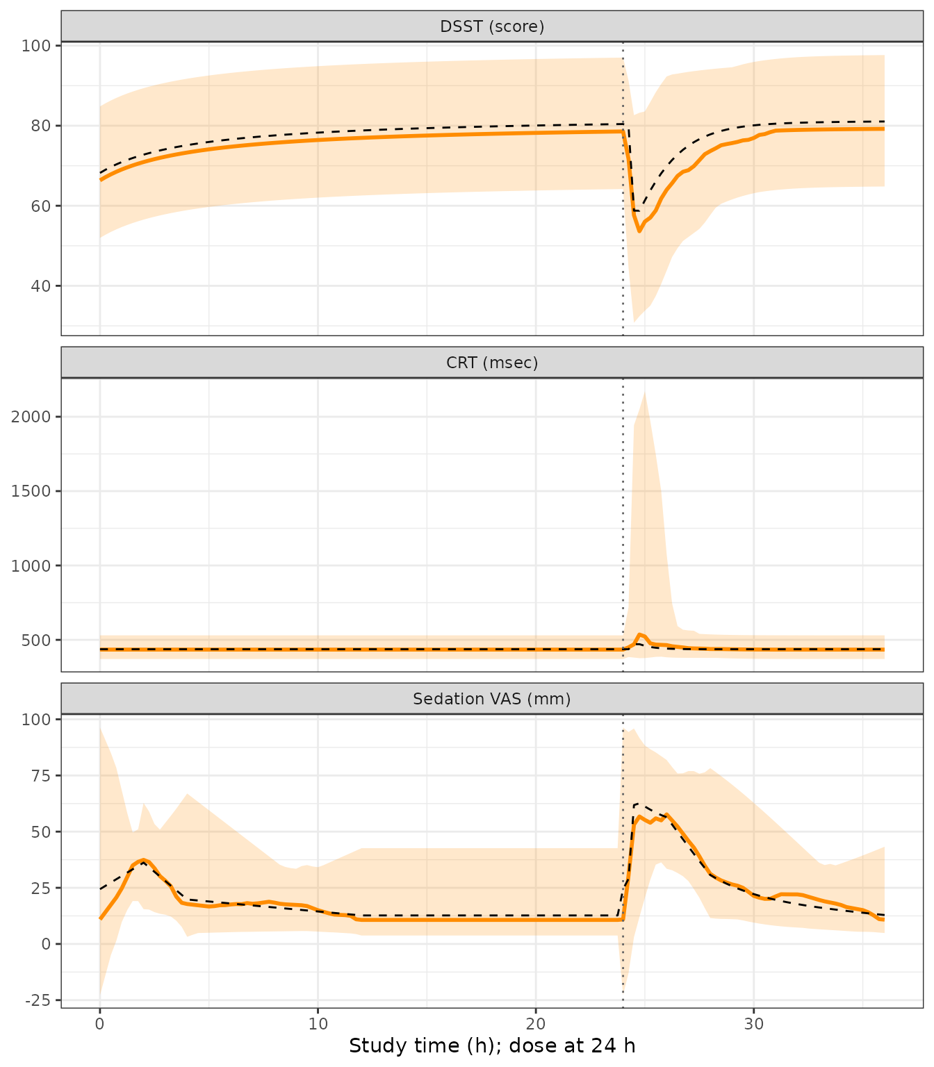

Simulated PD time courses. Ribbon = 5th-95th percentile of the simulated cohort, solid line = median, dashed line = the reference-subject typical-value profile. The vertical line marks dosing at t = 24 h. Replicates the layout of Kim 2026 Figure 2B-D.

Gate: return to baseline by 12 h after dosing

“At the reference age of 29.5 years, both DSST and CRT responses returned to baseline levels approximately 12 h after administration of zolpidem 10 mg (Figure S14).”

For DSST, “baseline” at 12 h post-dose is the learning-adjusted baseline elearn, not the constant BASE; for CRT it is rbase. Both are read off the typical-value solve.

t_end <- 36 # 12 h after the 24 h dose
d36 <- typ_dsst[typ_dsst$time == t_end, ][1, ]
c36 <- typ_crt[typ_crt$time == t_end, ][1, ]

dsst_recovery <- d36$DSST / d36$elearn
crt_recovery  <- c36$CRT  / c36$rbase

# Both endpoints must be within 1% of their own baseline at 12 h post-dose.
stopifnot(dsst_recovery > 0.99, crt_recovery < 1.01)

sprintf("At 12 h post-dose: DSST is %.2f%% of its learning-adjusted baseline; CRT is %.2f%% of its baseline.",
        100 * dsst_recovery, 100 * crt_recovery)
#> [1] "At 12 h post-dose: DSST is 99.99% of its learning-adjusted baseline; CRT is 100.00% of its baseline."

Figure: combined covariate effects on potency

Replicates Kim 2026 Figure 4A – typical DSST IC₅₀ as a joint function of weight and albumin, over the observed ranges of both.

grid_cov <- tidyr::expand_grid(
  WT  = seq(50, 83, length.out = 34),
  ALB = seq(3.9, 5.0, length.out = 23) * 10
) |>
  mutate(
    ic50 = 205 *
      (WT / 60.05)^ui_dsst$theta[["e_wt_ic50"]] *
      (1 + ui_dsst$theta[["e_alb_ic50"]] * (ALB * 0.1 - 4.4))
  )

# Cross-check one grid point against the solved model so the plotted surface is
# not an independently re-typed formula.
chk_point <- grid_cov[which.min(abs(grid_cov$WT - 78) + abs(grid_cov$ALB - 44)), ]
stopifnot(abs(
  chk_point$ic50 -
    205 * cov_multiplier(ui_dsst, "cov_ic50", list(WT = chk_point$WT, ALB = chk_point$ALB))
) < 1e-8)
#> ℹ omega/sigma items treated as zero: 'etalka', 'etalcl', 'etalmtt', 'etalfdepot', 'etalic50', 'etalrbase'

ggplot(grid_cov, aes(WT, ALB / 10)) +
  geom_raster(aes(fill = ic50)) +
  geom_contour(aes(z = ic50), colour = "white", linewidth = 0.3) +
  scale_fill_viridis_c(name = "IC50 (ug/L)") +
  labs(x = "Weight (kg)", y = "Albumin (g/dL)") +
  theme_bw()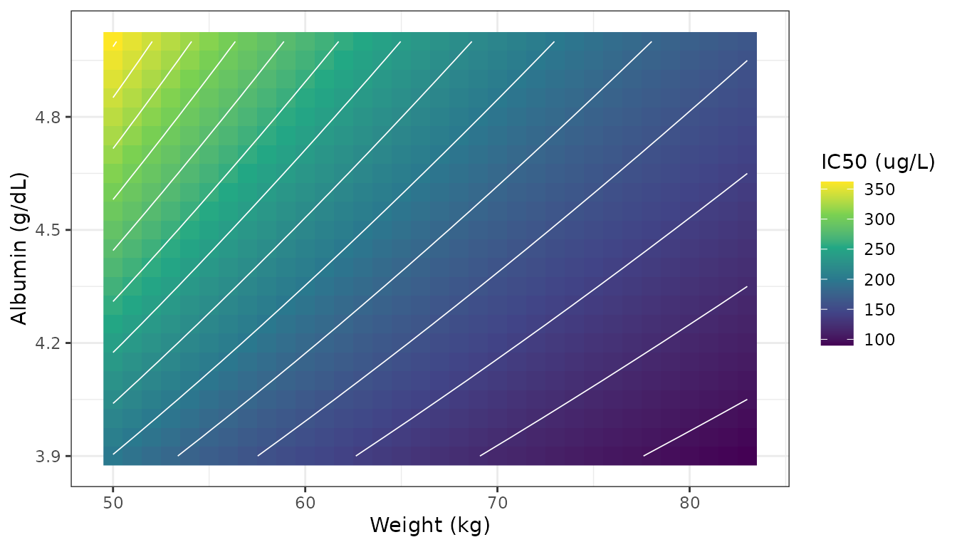

Typical DSST IC50 across the observed weight and albumin ranges, from the fixed effects of the final PK-DSST model. Replicates Kim 2026 Figure 4A.

Assumptions and deviations

Errata and source conflicts

Kim 2026 Table 3 footnote a drops an exponent. The footnote prints IC50,DSST (ug/L) = 205 x (Weight/60.05) x (1 + 0.541 x (Albumin - 4.4)), with weight entering linearly. The deposited control stream Data S2 gives the true form, IC50WEI = ((WEI/60.05)**THETA(18)) with THETA(18) = -1.57, i.e. a power term; the orphaned “-1.57” that trails the Table 3 abbreviations block in the published PDF is the dropped superscript. Table 3’s own “Effect of weight on IC₅₀” row also reports -1.57. The power form is what the model file encodes, and the forest-plot gate above settles it independently: Results 3.4 quotes 0.66 [0.59-0.74] at the 90th weight percentile, and (78.0/60.05)^-1.57 = 0.663, whereas the linear form printed in the footnote would give 1.30.
H₃ differs by one unit in the third digit. Kim 2026 Table 3 reports the third VAS baseline knot as 0.198 (SIR median 0.198) and Results 3.2.4 states the corresponding baseline as 19.8 mm; the Data S4 $THETA(13) entry is 0.199. The model file uses the paper’s 0.198, which is stated three times independently against the control stream’s once. The difference is 0.1 mm on a 100 mm scale.
Near-zero fixed residual-error components are retained. Each control stream builds a combined error, W = SQRT(prop^2 * IPRED^2 + add^2), and fixes the unused half at 1e-5 as a numerical guard. Kim 2026 Tables 2 and 3 report only the estimated half. The model files encode both, wrapping the 1e-5 term in fixed(), so that the encoded error model matches the deposited $ERROR block exactly.

Assumptions

Covariate distribution shapes. Kim 2026 Table 1 reports medians and ranges, not distributional shapes. The virtual cohort draws weight, albumin, age and baseline CRT from truncated normals centred on the published sex-specific medians with the range spanning about +/- 2 SD. The marginal medians and ranges therefore match Table 1, but the correlation structure between covariates does not: Figure S1 shows a correlated covariate matrix stratified by sex which is not reproducible from the published summaries. Any cohort-level percentile in this vignette should be read with that in mind; every published-value gate above is evaluated at fixed reference covariates and is unaffected.
Spline slope denominators use nominal times. Data S4 divides each spline segment by the difference of the actual observation times at the bracketing knots (CKT1..CKT4). Those equal the nominal 1, 2, 4 and 12 h whenever sampling is on schedule, and the model file writes them as the nominal values, since the actual per-subject times are not published.
Baseline VAS beyond the last knot. Data S4 assigns the flat value 100 * H4 only at exactly NCKT == 12, because no observation falls later. The model file holds the baseline flat at 100 * H4 for all times at or beyond 12 h, which is well-defined and agrees with the control stream everywhere the control stream is defined.
Stirling versus exact gamma normalisation. Data S1-S4 normalise the transit density with Stirling’s approximation, LNFAC = LOG(2.5066) + (NN + 0.5) * LOG(NN) - NN. rxode2’s builtin transit() evaluates the identical density but normalises with the exact lgamma(NN + 1). At NN = 19.4 the two differ by roughly 0.4% of the input rate, and the exact form is the more correct of the two; the AUC gate above confirms that the whole dose is still delivered.
Albumin unit conversion. The canonical ALB register unit is SI g/L while Kim 2026 calibrated its coefficients against US-convention g/dL. Each model file applies the register-mandated inline conversion alb_gdL <- ALB * 0.1 in model(), so the published coefficients are used unchanged and a model-data column of 44 g/L is the reference subject.
Half-life is not tuned to the published NCA. The model’s disposition half-life is 2.46 h by construction, about 18% shorter than the 2.9-3.1 h NCA mean quoted in the Introduction from the source clinical study. This follows from the published one-compartment structure and is left as-is.

Convention deviations

None. All four models pass checkModelConventions() with only the informational note that units$dosing (mg) and the units$concentration numerator (ug) differ in magnitude – the required 1000x scaling is applied explicitly in each model() block as Cc <- 1000 * central / vc, matching the control streams’ S2 = V2/1000.

Three covariate canonicals were registered with this extraction: CRT_BL, DSST_BL and VAS_SEDATION_BL.

#> 
#> ── Convention check: "Kim_2026_zolpidem" ───────────────────────────────────────
#> ℹ 1 info
#> 
#> ── units ──
#> 
#> ℹ [info] dosing_concentration: units$dosing ('mg') and units$concentration numerator ('ug') differ in magnitude; ensure scaling is applied in model().
#> suggestion: When dosing is mg but concentration is ug/mL (= mg/L), no
#> conversion is needed if volume is in L. Verify the relationship.
#> Kim_2026_zolpidem: 0 error(s), 0 warning(s)
#> 
#> ── Convention check: "Kim_2026_zolpidem_dsst" ──────────────────────────────────
#> ℹ 1 info
#> 
#> ── units ──
#> 
#> ℹ [info] dosing_concentration: units$dosing ('mg') and units$concentration numerator ('ug') differ in magnitude; ensure scaling is applied in model().
#> suggestion: When dosing is mg but concentration is ug/mL (= mg/L), no
#> conversion is needed if volume is in L. Verify the relationship.
#> Kim_2026_zolpidem_dsst: 0 error(s), 0 warning(s)
#> 
#> ── Convention check: "Kim_2026_zolpidem_crt" ───────────────────────────────────
#> ℹ 1 info
#> 
#> ── units ──
#> 
#> ℹ [info] dosing_concentration: units$dosing ('mg') and units$concentration numerator ('ug') differ in magnitude; ensure scaling is applied in model().
#> suggestion: When dosing is mg but concentration is ug/mL (= mg/L), no
#> conversion is needed if volume is in L. Verify the relationship.
#> Kim_2026_zolpidem_crt: 0 error(s), 0 warning(s)
#> 
#> ── Convention check: "Kim_2026_zolpidem_vas" ───────────────────────────────────
#> ℹ 1 info
#> 
#> ── units ──
#> 
#> ℹ [info] dosing_concentration: units$dosing ('mg') and units$concentration numerator ('ug') differ in magnitude; ensure scaling is applied in model().
#> suggestion: When dosing is mg but concentration is ug/mL (= mg/L), no
#> conversion is needed if volume is in L. Verify the relationship.
#> Kim_2026_zolpidem_vas: 0 error(s), 0 warning(s)

Model and source

Population

Source trace

Reconciling the reported %CV against the encoded variances

Virtual cohort

Pharmacokinetics

Simulation

Figure: plasma zolpidem concentration-time profile

PKNCA validation

Structural gate: AUC0-inf must equal Dose x F / CL, per subject

Comparison against the published non-compartmental analysis

Pharmacodynamics

Simulation

Gate: the potency rank order reported in the Discussion

Gate: the DSST learning effect at the time of dosing

Gate: the baseline VAS spline knots

Gate: the covariate forest plots (Kim 2026 Figure 3, Results 3.4)

Hard gate: power versus linear weight effect on DSST IC50

Figure: PD time courses

Gate: return to baseline by 12 h after dosing

Figure: combined covariate effects on potency

Assumptions and deviations

Errata and source conflicts

Assumptions

Convention deviations

Hard gate: power versus linear weight effect on DSST IC₅₀