Atazanavir + Ritonavir (Schipani 2013)
Source:vignettes/articles/Schipani_2013_atazanavir_ritonavir.Rmd
Schipani_2013_atazanavir_ritonavir.RmdModel and source
- Citation: Schipani A, Dickinson L, Boffito M, Austin R, Owen A, Back D, Khoo S, Davies G. Simultaneous Population Pharmacokinetic Modelling of Atazanavir and Ritonavir in HIV-Infected Adults and Assessment of Different Dose Reduction Strategies. J Acquir Immune Defic Syndr. 2013;62(1):60-66. doi:10.1097/QAI.0b013e3182737231.
- Description: Simultaneous one-compartment first-order-absorption popPK model for oral atazanavir (ATV) and ritonavir (RTV) in 30 HIV-infected adults receiving ATV/RTV 300/100 mg once daily, with a direct sigmoidal-Emax inhibition of ATV apparent clearance by RTV plasma concentration (Imax = 0.988, IC50 = 0.221 mg/L). Both drugs share a one-compartment structure with first-order absorption and an absorption lag time; ka values are fixed to the separate-model final estimates (ATV ka = 1.81 1/h, RTV ka = 0.898 1/h) because joint estimation produced numerical instability. Inter-individual variability is carried on V/F for both drugs and on CL/F for RTV (correlated with V/F RTV, rho = 0.75); ATV CL/F is fitted without IIV. Demographic covariates and tenofovir co-administration were tested and none retained (Schipani 2013).
- Article: https://doi.org/10.1097/QAI.0b013e3182737231
Population
Schipani 2013 pooled data from three previously published studies of HIV-infected adults treated with the licensed atazanavir/ritonavir (ATV/RTV) 300/100 mg once-daily regimen, all enrolled at a single UK study centre (St Stephen’s Centre, Chelsea and Westminster Foundation Trust, London). 30 patients contributed 288 ATV and 312 RTV plasma concentrations on a single sampling occasion (median 11 samples per patient). The cohort was 27/30 male, median age 43 years (range 22-62), median body weight 75.5 kg (range 46-110); the majority were white with 5 Black-Africans and 3 Hispanics. 5/30 subjects were co-administered tenofovir 300 mg once daily. Baseline HIV viral load was a median of 61 copies/mL (range <50-72).
Demographic covariates (gender, ethnicity, body weight, age) and tenofovir co-administration were tested via generalized additive modelling on the basic separate-drug models; none was retained in the final combined model (Schipani 2013 Results, Discussion). The packaged model therefore exposes no covariate columns.
The same information is available programmatically via
readModelDb("Schipani_2013_atazanavir_ritonavir")()$meta$population.
Source trace
Per-parameter origin is recorded as an in-file comment next to each
ini() entry in
inst/modeldb/specificDrugs/Schipani_2013_atazanavir_ritonavir.R.
The table below collects them for review.
| Equation / parameter | Value | Source location |
|---|---|---|
| Atazanavir CL/F (in absence of RTV) | 16.6 L/h (RSE 7%) | Table 2 |
| Atazanavir V/F | 106 L (RSE 7%) | Table 2 |
| Atazanavir ka (FIXED) | 1.81 1/h | Table 2 (fixed from separate-model final value in Table 1) |
| Atazanavir Tlag | 0.87 h (RSE 2%) | Table 2 |
| Ritonavir CL/F | 13.2 L/h (RSE 12%) | Table 2 |
| Ritonavir V/F | 124 L (RSE 11%) | Table 2 |
| Ritonavir ka (FIXED) | 0.898 1/h | Table 2 (fixed from separate-model final value in Table 1) |
| Ritonavir Tlag | 1.05 h (RSE 1%) | Table 2 |
| Imax (maximum inhibition of ATV CL/F) | 0.988 (RSE 1%) | Table 2 |
| IC50 (RTV concentration for 50% Imax) | 0.221 mg/L (RSE 13%) | Table 2 |
| IIV V/F ATV | 53% CV (RSE 23%) | Table 2 |
| IIV CL/F RTV | 77% CV (RSE 14%) | Table 2 |
| IIV V/F RTV | 73% CV (RSE 16%) | Table 2 |
| Correlation (CL/F RTV, V/F RTV) | 0.75 (RSE 13%) | Table 2 |
| Proportional residual ATV | 63% (RSE 18%) | Table 2 |
| Proportional residual RTV | 73% (RSE 5%) | Table 2 |
| Direct-effect inhibition equation |
CL_ATV(t) = CL0_ATV * (1 - I(t));
I(t) = Imax * C_RTV / (IC50 + C_RTV)
|
Methods, “Population PK Modelling” section |
Virtual cohort
Original observed data are not publicly available. The simulations below build a virtual cohort of 200 subjects per dosing regimen, mirroring the four dose-reduction scenarios evaluated in the paper (licensed 300/100 mg plus 300/50, 200/100, and 200/50 mg ATV/RTV once daily). Subjects have no covariates beyond ID because the final model retains no covariate effects.
set.seed(20260520)

n_per_arm <- 200L
tau       <- 24                     # dosing interval (h)
n_doses   <- 14L                    # 14 daily doses -> steady state
obs_times <- sort(unique(c(
  seq(0, tau,            length.out = 25),               # dense over the first interval
  seq(tau, (n_doses - 1) * tau,  by = tau),              # daily troughs through day 14
  (n_doses - 1) * tau + seq(0, tau, length.out = 49)     # dense over the steady-state day-14 interval
)))

regimens <- tibble::tribble(
  ~regimen,     ~atv_mg, ~rtv_mg,
  "300/100 mg",      300,     100,
  "300/50 mg",       300,      50,
  "200/100 mg",      200,     100,
  "200/50 mg",       200,      50
)

make_cohort <- function(n, atv_mg, rtv_mg, regimen, id_offset) {
  ids <- id_offset + seq_len(n)
  dose_times <- seq(0, (n_doses - 1) * tau, by = tau)

  dose_atv <- tidyr::expand_grid(id = ids, time = dose_times) |>
    dplyr::mutate(amt = atv_mg, cmt = "depot",     evid = 1L)
  dose_rtv <- tidyr::expand_grid(id = ids, time = dose_times) |>
    dplyr::mutate(amt = rtv_mg, cmt = "depot_rtv", evid = 1L)

  obs <- tidyr::expand_grid(id = ids, time = obs_times,
                            cmt = c("Cc", "Cc_rtv")) |>
    dplyr::mutate(amt = 0, evid = 0L)

  dplyr::bind_rows(dose_atv, dose_rtv, obs) |>
    dplyr::mutate(regimen = regimen) |>
    dplyr::arrange(id, time, evid)
}

id_seed <- 0L
events_list <- list()
for (i in seq_len(nrow(regimens))) {
  r <- regimens[i, ]
  events_list[[i]] <- make_cohort(n_per_arm, r$atv_mg, r$rtv_mg, r$regimen,
                                  id_offset = id_seed)
  id_seed <- id_seed + n_per_arm
}
events <- dplyr::bind_rows(events_list)
stopifnot(!anyDuplicated(unique(events[, c("id", "time", "evid", "cmt")])))
Simulation
mod <- readModelDb("Schipani_2013_atazanavir_ritonavir")

# Stochastic VPC with the published IIV (RTV CL+V correlated, ATV V/F univariate).
sim <- rxode2::rxSolve(mod, events = events,
                       keep = c("regimen")) |>
  as.data.frame()

# Deterministic (typical-value) simulation for Figure 3 replication.
mod_typical <- rxode2::zeroRe(mod)
sim_typical <- rxode2::rxSolve(mod_typical, events = events,
                               keep = c("regimen")) |>
  as.data.frame()
#> ℹ omega/sigma items treated as zero: 'etalvc', 'etalcl_rtv', 'etalvc_rtv'
#> Warning: multi-subject simulation without without 'omega'
Replicate published figures
Figure 3 – ATV concentration-time profile at three dose regimens
Schipani 2013 Figure 3 plots the simulated mean plasma ATV concentration over a 24-h dosing interval at steady state for ATV/RTV 300/50, 200/50, and 200/100 mg once daily, together with the licensed 300/100 mg reference profile. We reproduce the typical-value (no-IIV) curves directly from the packaged model. Stochastic envelopes (median, 5th and 95th percentiles) are overlaid to convey the population spread that drives the Cmin distribution discussed in the paper Results.
day14_start <- (n_doses - 1) * tau
ss_window <- sim |>
  dplyr::filter(time >= day14_start) |>
  dplyr::mutate(t_h = time - day14_start)
ss_window_typical <- sim_typical |>
  dplyr::filter(time >= day14_start) |>
  dplyr::mutate(t_h = time - day14_start)

vpc_atv <- ss_window |>
  dplyr::group_by(regimen, t_h) |>
  dplyr::summarise(
    Q05 = quantile(Cc, 0.05, na.rm = TRUE),
    Q50 = quantile(Cc, 0.50, na.rm = TRUE),
    Q95 = quantile(Cc, 0.95, na.rm = TRUE),
    .groups = "drop"
  )

typ_atv <- ss_window_typical |>
  dplyr::distinct(regimen, t_h, Cc)

ggplot() +
  geom_ribbon(data = vpc_atv,
              aes(t_h, ymin = Q05, ymax = Q95, fill = regimen),
              alpha = 0.20) +
  geom_line(data = vpc_atv, aes(t_h, Q50, colour = regimen), linewidth = 0.6) +
  geom_line(data = typ_atv, aes(t_h, Cc, colour = regimen),
            linewidth = 1.0, linetype = "dashed") +
  scale_y_log10() +
  labs(x = "Time after dose (h)", y = "Atazanavir plasma concentration (mg/L)",
       title = "Figure 3 -- ATV steady-state concentration-time profile by regimen",
       caption = paste0("Replicates Figure 3 of Schipani 2013. Solid line: ",
                        "stochastic median (n = ", n_per_arm,
                        " per regimen). Dashed line: typical-value (no-IIV) profile. ",
                        "Ribbon: 5th-95th percentile."))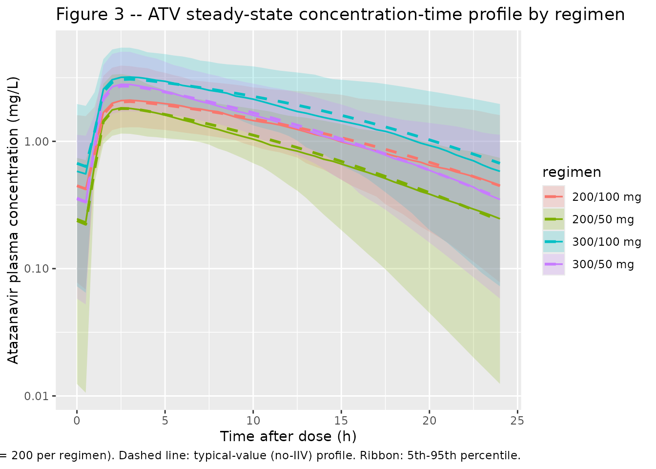
PKNCA validation
PKNCA computes steady-state non-compartmental Cmax, Cmin, and
AUC0-tau over the last (14th) dosing interval for ATV and RTV at each
regimen. The PKNCA formula stratifies by regimen so
per-regimen mean values can be compared against the paper’s reported
simulated trough means.
nca_window_atv <- sim |>
  dplyr::filter(time >= day14_start, time <= day14_start + tau) |>
  dplyr::filter(!is.na(Cc)) |>
  dplyr::distinct(id, time, regimen, .keep_all = TRUE) |>
  dplyr::select(id, time, Cc, regimen)

dose_df <- events |>
  dplyr::filter(evid == 1, cmt == "depot",
                time == max(time[evid == 1L & cmt == "depot"])) |>
  dplyr::distinct(id, time, amt, regimen)

conc_atv <- PKNCA::PKNCAconc(nca_window_atv,
                             Cc ~ time | regimen + id,
                             concu = "mg/L", timeu = "h")
dose_atv <- PKNCA::PKNCAdose(dose_df, amt ~ time | regimen + id,
                             doseu = "mg")

intervals_ss <- data.frame(
  start  = day14_start,
  end    = day14_start + tau,
  cmax   = TRUE,
  cmin   = TRUE,
  tmax   = TRUE,
  auclast = TRUE,
  cav    = TRUE
)

nca_res_atv <- PKNCA::pk.nca(PKNCA::PKNCAdata(conc_atv, dose_atv,
                                              intervals = intervals_ss))
nca_summary_atv <- as.data.frame(summary(nca_res_atv))
knitr::kable(nca_summary_atv,
caption = "Simulated steady-state NCA -- atazanavir, by regimen.")| Interval Start | Interval End | regimen | N | AUClast (h*mg/L) | Cmax (mg/L) | Cmin (mg/L) | Tmax (h) | Cav (mg/L) |
|---|---|---|---|---|---|---|---|---|
| 312 | 336 | 200/100 mg | 200 | 30.9 [35.3] | 2.19 [35.0] | 0.363 [150] | 3.00 [2.00, 3.50] | 1.29 [35.3] |
| 312 | 336 | 200/50 mg | 200 | 22.5 [28.6] | 1.89 [34.1] | 0.177 [211] | 2.50 [2.00, 3.50] | 0.936 [28.6] |
| 312 | 336 | 300/100 mg | 200 | 44.7 [33.7] | 3.26 [31.4] | 0.484 [163] | 3.00 [2.00, 3.50] | 1.86 [33.7] |
| 312 | 336 | 300/50 mg | 200 | 34.2 [26.9] | 2.83 [34.3] | 0.299 [125] | 2.50 [2.00, 3.50] | 1.43 [26.9] |
nca_window_rtv <- sim |>
  dplyr::filter(time >= day14_start, time <= day14_start + tau) |>
  dplyr::filter(!is.na(Cc_rtv)) |>
  dplyr::distinct(id, time, regimen, .keep_all = TRUE) |>
  dplyr::select(id, time, Cc_rtv, regimen)

dose_df_rtv <- events |>
  dplyr::filter(evid == 1, cmt == "depot_rtv",
                time == max(time[evid == 1L & cmt == "depot_rtv"])) |>
  dplyr::distinct(id, time, amt, regimen)

conc_rtv <- PKNCA::PKNCAconc(nca_window_rtv,
                             Cc_rtv ~ time | regimen + id,
                             concu = "mg/L", timeu = "h")
dose_rtv <- PKNCA::PKNCAdose(dose_df_rtv, amt ~ time | regimen + id,
                             doseu = "mg")

nca_res_rtv <- PKNCA::pk.nca(PKNCA::PKNCAdata(conc_rtv, dose_rtv,
                                              intervals = intervals_ss))
nca_summary_rtv <- as.data.frame(summary(nca_res_rtv))
knitr::kable(nca_summary_rtv,
caption = "Simulated steady-state NCA -- ritonavir, by regimen.")| Interval Start | Interval End | regimen | N | AUClast (h*mg/L) | Cmax (mg/L) | Cmin (mg/L) | Tmax (h) | Cav (mg/L) |
|---|---|---|---|---|---|---|---|---|
| 312 | 336 | 200/100 mg | 200 | 7.65 [74.4] | 0.685 [68.2] | 0.0636 [207] | 3.50 [3.00, 4.00] | 0.319 [74.4] |
| 312 | 336 | 200/50 mg | 200 | 3.57 [82.7] | 0.318 [74.6] | 0.0307 [205] | 3.50 [3.00, 4.00] | 0.149 [82.7] |
| 312 | 336 | 300/100 mg | 200 | 7.09 [76.6] | 0.656 [69.2] | 0.0516 [276] | 3.50 [2.50, 4.00] | 0.295 [76.6] |
| 312 | 336 | 300/50 mg | 200 | 3.81 [73.7] | 0.335 [72.8] | 0.0345 [155] | 3.50 [3.00, 4.00] | 0.159 [73.7] |
Comparison against published simulated values
Schipani 2013 reports simulated mean ATV trough concentrations across 1,000 virtual subjects per regimen (paper Results, “Simulations of the Dose Reduction Strategy”). The packaged model is exercised on 200 subjects per regimen here for vignette wall-clock economy; relative differences vs the licensed regimen should match the paper’s reported ratios (45%, 63%, and 33% reductions for 300/50, 200/50, and 200/100 mg respectively).
troughs <- sim |>
  dplyr::filter(time == day14_start + tau) |>
  dplyr::group_by(regimen) |>
  dplyr::summarise(
    mean_ctrough_mgL = mean(Cc, na.rm = TRUE),
    sd_ctrough_mgL   = sd(Cc,   na.rm = TRUE),
    pct_below_MEC    = 100 * mean(Cc < 0.15, na.rm = TRUE),
    .groups = "drop"
  )

ref_mean <- troughs$mean_ctrough_mgL[troughs$regimen == "300/100 mg"]
troughs <- troughs |>
  dplyr::mutate(
    pct_change_vs_300_100 = 100 * (mean_ctrough_mgL - ref_mean) / ref_mean,
    published_mean_mgL = c(0.80, 0.437, 0.520, 0.303)[
      match(regimen, c("300/100 mg", "300/50 mg", "200/100 mg", "200/50 mg"))
    ],
    published_pct_change = c(0, -45, -33, -63)[
      match(regimen, c("300/100 mg", "300/50 mg", "200/100 mg", "200/50 mg"))
    ]
  )

knitr::kable(troughs,
             caption = paste0("Simulated ATV trough comparison vs Schipani 2013 ",
                              "Results (Simulations of the Dose Reduction Strategy). ",
                              "MEC = 0.15 mg/L (paper cites this as the recommended ",
"minimum effective concentration for boosted ATV)."))| regimen | mean_ctrough_mgL | sd_ctrough_mgL | pct_below_MEC | pct_change_vs_300_100 | published_mean_mgL | published_pct_change |
|---|---|---|---|---|---|---|
| 200/100 mg | 0.5865990 | 0.5638285 | 15.0 | -26.33245 | 0.520 | -33 |
| 200/50 mg | 0.3119166 | 0.2990072 | 31.5 | -60.82822 | 0.303 | -63 |
| 300/100 mg | 0.7962787 | 0.7290383 | 11.0 | 0.00000 | 0.800 | 0 |
| 300/50 mg | 0.4409834 | 0.3326797 | 16.0 | -44.61946 | 0.437 | -45 |
Assumptions and deviations
- Atazanavir CL/F is fitted without IIV in the packaged model. This matches the paper’s final combined model exactly (Schipani 2013 Discussion: “the addition of IIV on ATV CL/F contributed to the instability of the model … thus IIV on ATV CL/F was not included in the final model”). The simulated between-subject variability in ATV exposure therefore arises entirely from (a) ATV V/F variability (53% CV), (b) ritonavir CL/V variability (77% / 73% CV, rho = 0.75) propagating through the sigmoidal inhibition term, and (c) proportional residual error.
-
ka values for both drugs are FIXED to the separate-model
final estimates (ATV 1.81 1/h, RTV 0.898 1/h). The paper holds
these parameters constant because joint estimation produced numerical
instability (Schipani 2013 Results). They are encoded with
fixed()inini()so downstream users can see the constraint. -
Bioavailability F is not in the model (F = 1 by
default). The paper parameterises CL/F and V/F directly without
resolving F; the rxode2/nlmixr2 default
f(depot) = 1reproduces this. - MEC threshold of 0.15 mg/L is used in the trough-comparison table. The paper refers to a recommended ATV minimum effective concentration (MEC) and quotes the proportion of subjects below it for each dose-reduction regimen (6% at 300/100 mg, 17.8% at 300/50 mg, 33.9% at 200/50 mg, 15.3% at 200/100 mg). The 0.15 mg/L value used here is the protein-binding-adjusted IC50 commonly cited in the HIV pharmacotherapy literature; the paper Results section does not state the exact mg/L cut-off. Adjust the threshold if matching a different published MEC convention.
-
Simulated cohort size 200 per regimen (vs the
paper’s 1,000) is a vignette-time budget choice. Relative differences
across regimens are stable at this n; absolute Cmin standard deviations
may be noisier than the published ones. Increase
n_per_armfor a closer reproduction of the simulated SDs in the paper’s Results section. - No errata or corrigenda for the source paper were located via the publisher landing page or PubMed at the time of extraction. The Europe PMC funders-group manuscript and the final published article (J Acquir Immune Defic Syndr 2013;62(1):60-66) are identical for the parameter values used here.