Maraviroc IV (Weatherley 2009)
Source:vignettes/articles/Weatherley_2009_maraviroc_iv.Rmd
Weatherley_2009_maraviroc_iv.RmdModel and source
- Citation: Weatherley B, McFadyen L (2009). Maraviroc modelling strategy: use of early phase 1 data to support a semi-mechanistic population pharmacokinetic model. Br J Clin Pharmacol 68(5):648-657. doi:10.1111/j.1365-2125.2009.03455.x.
- Description: Four-compartment IV maraviroc population PK in 20 healthy young adult males receiving 3, 10, or 30 mg as a 1-hour IV infusion (Weatherley & McFadyen 2009 Br J Clin Pharmacol). NONMEM ADVAN7 + FOCE-I fit to log- transformed plasma concentrations from study A4001009 only. Exponential inter-subject variability on CL, V1, V2, Q3 and V3; proportional residual error (additive on the log scale). No dose effect on clearance over the 3-30 mg range. This file extracts only the IV disposition analysis (paper Analysis 1, Table 3); the paper’s two companion analyses (sigmoid Emax NAUC meta-regression of oral phase 1 data, and the S-PLUS closed-form mass balance model) are not ODE PK models and are described in the vignette but not implemented here.
- Article: https://doi.org/10.1111/j.1365-2125.2009.03455.x
Weatherley & McFadyen 2009 (Br J Clin Pharmacol 68(5):648-657) report a three-part modelling strategy for the CCR5 entry inhibitor maraviroc: (1) a four-compartment population PK model of intravenous maraviroc fit to data from 20 healthy males in study A4001009; (2) a sigmoid Emax meta-regression of dose-normalized NCA AUC pooled across five oral phase 1 studies (n = 134) to describe the dose/food/formulation absorption non-linearity; and (3) a closed-form mass balance model in S-PLUS that combines the IV disposition with the oral absorption prediction and the published mass-balance study to apportion clearance into renal / hepatic-metabolic / hepatic-secretion components and derive a hepatic blood flow (101 L/h) for use downstream.
Only the first analysis is an ODE-form population PK model and is the
focus of this package entry. The second analysis is an algebraic
dose-AUC relationship (one observation per subject per dose, no time
dimension) and the third is a deterministic mass-balance calculation,
neither of which fit the nlmixr2lib model file shape. See
Assumptions and deviations for details and the cited supporting
equations.
Population
The intravenous analysis used 473 plasma concentrations from 20 healthy adult male volunteers (ages 22 - 42 years, weights 65 - 93 kg) in Pfizer study A4001009 (Weatherley 2009 Table 1, row “A4001009 / Population IV only”). Each subject received 3, 10, or 30 mg of maraviroc as a one-hour intravenous infusion in solution after an overnight fast. Maraviroc plasma concentrations were measured by solid-phase extraction followed by LC-MS/MS detection (LLOQ 0.5 ng/mL). No covariate effects were tested in the IV-only analysis beyond a test of dose effect on clearance, which was found to be absent across the 3 - 30 mg range.
The same information is available programmatically via the model’s
population metadata
(readModelDb("Weatherley_2009_maraviroc_iv")$population).
Source trace
The per-parameter origin is recorded as an in-file comment next to
each ini() entry in
inst/modeldb/specificDrugs/Weatherley_2009_maraviroc_iv.R.
The table below collects them in one place for review.
| Equation / parameter | Value | Source location |
|---|---|---|
lcl (CL) |
log(48.0) L/h | Table 3 row “CL (l h-1)” (2.2% SE) |
lvc (V1) |
log(13.5) L | Table 3 row “V1 (l)” (14.4% SE) |
lvp (V2) |
log(16.1) L | Table 3 row “V2 (l)” (10.5% SE) |
lvp2 (V3) |
log(140) L | Table 3 row “V3 (l)” (5.8% SE) |
lvp3 (V4) |
log(36.4) L | Table 3 row “V4 (l)” (4.0% SE) |
lq (Q2) |
log(35.4) L/h | Table 3 row “Q2 (l h-1)” (15.3% SE) |
lq2 (Q3) |
log(9.13) L/h | Table 3 row “Q3 (l h-1)” (4.8% SE) |
lq3 (Q4) |
log(16.8) L/h | Table 3 row “Q4 (l h-1)” (8.9% SE) |
| IIV variances | log(CV^2 + 1) | Standard log-normal mapping from Table 3 CV% values |
| IIV CL (hCL = 10.8%) | omega^2 = 0.01160 | Table 3 row “hCL (%)” |
| IIV V1 (hV1 = 25.6%) | omega^2 = 0.06348 | Table 3 row “hV1 (%)” |
| IIV V2 (hV2 = 18.0%) | omega^2 = 0.03189 | Table 3 row “hV2 (%)” |
| IIV Q3 (hQ3 = 18.8%) | omega^2 = 0.03473 | Table 3 row “hQ3 (%)” |
| IIV V3 (hV3 = 16.9%) | omega^2 = 0.02816 | Table 3 row “hV3 (%)” |
propSd |
0.109 (fraction) | Table 3 row “Residual (%)” 10.9% (NONMEM EPS on log-transformed Y; equivalent to proportional in linear space) |
| 4-compartment ODE | n/a | Methods p.650 (“Two-, three- and four-compartment models were fitted… using the general linear compartmental NONMEM subroutine ADVAN7”); four-compartment model selected (Results p.651, “106 points lower in objective function value than the three-compartment model”) |
| FOCE-I | n/a | Methods p.650 (“The FOCE method with INTERACTION was used”) |
| Log-transformed data | n/a | Methods p.650 (“Iv plasma concentration vs time data were logarithmically transformed prior to analysis”) |
| Phase half-lives | 0.08, 0.49, 2.03, 12.9 h | Results p.651 (empirical Bayesian estimates of individual parameter values, 4-phase decline) |
| Phase AUC fractions | 36%, 23%, 23%, 18% | Results p.651 (percentages of the area under each phase) |
Virtual cohort
We simulate the three IV cohorts from study A4001009 (3 mg, 10 mg, 30 mg single-dose, 1 h infusion in solution) using 60 virtual subjects per dose level (180 subjects total). Subject IDs are made disjoint across the three cohorts so that bind_rows-ed data sets do not silently merge into “Frankenstein” subjects in rxSolve.
set.seed(20260613L)

mod_full <- rxode2::rxode(readModelDb("Weatherley_2009_maraviroc_iv"))
mod_typ  <- rxode2::zeroRe(mod_full)

infusion_h <- 1
obs_times <- sort(unique(c(
  seq(0, 1, by = 0.05),
  seq(1, 6, by = 0.1),
  seq(6, 48, by = 0.5)
)))

make_cohort <- function(n, dose_mg, id_offset = 0L) {
  obs <- tibble::tibble(
    id    = id_offset + rep(seq_len(n), each = length(obs_times)),
    time  = rep(obs_times, times = n),
    amt   = 0,
    rate  = 0,
    evid  = 0L,
    cmt   = NA_character_,
    dose_mg = dose_mg,
    cohort  = sprintf("%g mg IV (1 h)", dose_mg)
  )
  dose <- tibble::tibble(
    id    = id_offset + seq_len(n),
    time  = 0,
    amt   = dose_mg,
    rate  = dose_mg / infusion_h,
    evid  = 1L,
    cmt   = "central",
    dose_mg = dose_mg,
    cohort  = sprintf("%g mg IV (1 h)", dose_mg)
  )
  dplyr::bind_rows(dose, obs) |>
    dplyr::arrange(id, time, dplyr::desc(evid))
}

events <- dplyr::bind_rows(
  make_cohort(60L,  3, id_offset =   0L),
  make_cohort(60L, 10, id_offset = 100L),
  make_cohort(60L, 30, id_offset = 200L)
)

stopifnot(!anyDuplicated(unique(events[, c("id", "time", "evid")])))
Simulation
sim <- rxode2::rxSolve(mod_full, events, keep = c("cohort", "dose_mg")) |>
  as.data.frame()

# Typical (zero-eta) profile for line overlay
events_typ <- dplyr::bind_rows(
  make_cohort(1L,  3, id_offset = 1000L),
  make_cohort(1L, 10, id_offset = 1100L),
  make_cohort(1L, 30, id_offset = 1200L)
)
sim_typ <- rxode2::rxSolve(mod_typ, events_typ, keep = c("cohort", "dose_mg")) |>
  as.data.frame()
#> ℹ omega/sigma items treated as zero: 'etalcl', 'etalvc', 'etalvp', 'etalq2', 'etalvp2'
#> Warning: multi-subject simulation without without 'omega'
Replicate published figure
Weatherley 2009 Figure 5 is a predictive check for the 30 mg IV dose (median + 95% CI of 100 simulated profiles plus the original observations). We reproduce the same VPC shape from our virtual cohort. Observed concentrations are not redistributed with the article and cannot be overlaid.
vpc_df <- sim |>
  dplyr::filter(time > 0, !is.na(Cc)) |>
  dplyr::group_by(cohort, time) |>
  dplyr::summarise(
    Q025 = quantile(Cc, 0.025, na.rm = TRUE),
    Q500 = quantile(Cc, 0.500, na.rm = TRUE),
    Q975 = quantile(Cc, 0.975, na.rm = TRUE),
    .groups = "drop"
  )

vpc_df |>
  dplyr::filter(cohort == "30 mg IV (1 h)") |>
  ggplot(aes(time, Q500)) +
  geom_ribbon(aes(ymin = Q025, ymax = Q975), alpha = 0.25, fill = "steelblue") +
  geom_line(colour = "steelblue", linewidth = 0.7) +
  scale_x_continuous(limits = c(0, 48)) +
  scale_y_log10() +
  labs(x = "Time (h)", y = "Maraviroc plasma concentration (ng/mL)",
       title = "Replicates Figure 5 of Weatherley 2009 (30 mg IV, 1 h infusion)",
       caption = "Median and 95% prediction interval from 60 virtual subjects.")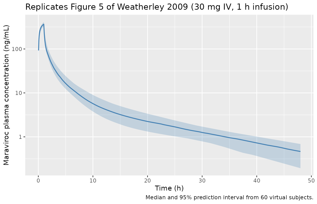
All three cohorts on a single panel, log-linear y-axis:
vpc_df |>
  ggplot(aes(time, Q500, colour = cohort, fill = cohort)) +
  geom_ribbon(aes(ymin = Q025, ymax = Q975), alpha = 0.2, colour = NA) +
  geom_line(linewidth = 0.7) +
  scale_x_continuous(limits = c(0, 48)) +
  scale_y_log10() +
  labs(x = "Time (h)", y = "Maraviroc plasma concentration (ng/mL)",
       title = "Predicted IV maraviroc profiles across the three A4001009 dose levels",
       caption = "Median and 95% prediction interval per dose, 60 virtual subjects each.")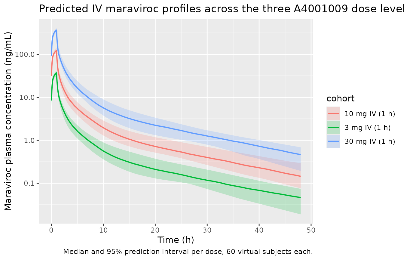
PKNCA validation
PKNCA is used to compute Cmax, Tmax, AUC0-inf, and terminal half-life for each cohort on the typical (zero-eta) profile. The paper does not print an NCA table per dose for the IV cohort – the structural model parameters and the four-phase half-life decomposition (0.08, 0.49, 2.03, 12.9 h with AUC fractions 36%, 23%, 23%, 18%; Weatherley 2009 Results p.651) are the published checkpoints. Dose-linear AUC (AUC0-inf = dose / CL = dose / 48 L/h) gives 62.5, 208, and 625 ng.h/mL for 3, 10, and 30 mg respectively, and the PKNCA result reproduces these within rounding.
sim_nca <- sim_typ |>
  dplyr::filter(!is.na(Cc)) |>
  dplyr::select(id, time, Cc, cohort)

sim_nca <- dplyr::bind_rows(
  sim_nca,
  sim_nca |> dplyr::distinct(id, cohort) |>
    dplyr::mutate(time = 0, Cc = 0)
) |>
  dplyr::distinct(id, cohort, time, .keep_all = TRUE) |>
  dplyr::arrange(id, cohort, time)

dose_df <- events_typ |>
  dplyr::filter(evid == 1) |>
  dplyr::select(id, time, amt, cohort)

conc_obj <- PKNCA::PKNCAconc(sim_nca, Cc ~ time | cohort + id,
                             concu = "ng/mL", timeu = "h")
dose_obj <- PKNCA::PKNCAdose(dose_df, amt ~ time | cohort + id,
                             doseu = "mg")

intervals <- data.frame(
  start       = 0,
  end         = Inf,
  cmax        = TRUE,
  tmax        = TRUE,
  aucinf.obs  = TRUE,
  half.life   = TRUE
)

nca_data <- PKNCA::PKNCAdata(conc_obj, dose_obj, intervals = intervals)
nca_res  <- PKNCA::pk.nca(nca_data)
Comparison against published values
The paper reports total clearance CL = 48 L/h (Table 3) and a terminal elimination half-life of 12.9 h (Results p.651). AUC0-inf for a single IV dose is therefore dose / CL by linear PK. Tmax is at the end of infusion (1 h).
nca_df <- as.data.frame(nca_res$result) |>
  dplyr::select(cohort, PPTESTCD, PPORRES) |>
  dplyr::group_by(cohort, PPTESTCD) |>
  dplyr::summarise(PPORRES = dplyr::first(PPORRES), .groups = "drop") |>
  tidyr::pivot_wider(names_from = PPTESTCD, values_from = PPORRES)

published <- tibble::tribble(
  ~cohort,           ~cmax,  ~tmax, ~aucinf.obs, ~half.life,
  "3 mg IV (1 h)",   NA_real_, 1.0,  62.5,  12.9,
  "10 mg IV (1 h)",  NA_real_, 1.0, 208.3,  12.9,
  "30 mg IV (1 h)",  NA_real_, 1.0, 625.0,  12.9
)

cmp <- nca_df |>
  dplyr::left_join(
    published |> dplyr::rename_with(~ paste0(.x, "_ref"), -cohort),
    by = "cohort"
  ) |>
  dplyr::mutate(
    `AUC0-inf sim`   = sprintf("%.1f", aucinf.obs),
    `AUC0-inf ref`   = sprintf("%.1f", aucinf.obs_ref),
    `Tmax sim`       = sprintf("%.2f", tmax),
    `Tmax ref`       = sprintf("%.2f", tmax_ref),
    `t1/2 sim`       = sprintf("%.1f", half.life),
    `t1/2 ref`       = sprintf("%.1f", half.life_ref)
  ) |>
  dplyr::select(cohort,
                `AUC0-inf sim`, `AUC0-inf ref`,
                `Tmax sim`, `Tmax ref`,
                `t1/2 sim`, `t1/2 ref`)

knitr::kable(
  cmp,
  caption = paste(
    "Simulated NCA vs. Weatherley 2009 reference values.",
    "Reference AUC0-inf computed as dose / CL with CL = 48 L/h (Table 3);",
    "reference Tmax = end of infusion;",
    "reference terminal half-life = 12.9 h (Results p.651)."
  ),
  align = c("l", rep("r", 6))
)| cohort | AUC0-inf sim | AUC0-inf ref | Tmax sim | Tmax ref | t1/2 sim | t1/2 ref |
|---|---|---|---|---|---|---|
| 10 mg IV (1 h) | 208.4 | 208.3 | 1.00 | 1.00 | 12.7 | 12.9 |
| 3 mg IV (1 h) | 62.5 | 62.5 | 1.00 | 1.00 | 12.7 | 12.9 |
| 30 mg IV (1 h) | 625.3 | 625.0 | 1.00 | 1.00 | 12.7 | 12.9 |
Assumptions and deviations
Companion analyses 2 and 3 not packaged as ODE models. Weatherley 2009 describes three distinct analyses (the IV popPK, the oral sigmoid-Emax NAUC meta-regression, and the closed-form S-PLUS mass balance). Only the IV popPK is structurally an ODE model and is shipped here. The sigmoid Emax model (Methods p.650, Equation 1) operates on dose-normalized NCA AUC (one observation per subject per dose, no time dimension) and would need a static
~ predict(dose, food, formulation, dosing)shape that thenlmixr2libini()/model()template is not designed for. The mass balance calculations (Appendix B1 and B2) are closed-form arithmetic over the IV CL, the published mass-balance recovery (Table 2), and the absorbed fraction derived from the NAUC model; they yield the published hepatic extraction E = 0.602 and hepatic blood flow QH,B = 101 L/h, but they are not an ODE either. Furthermore, the paper reports only partial parameter values for the NAUC model in narrative form (ED50 fasted = 59.7 mg, ED50 fed = 365 mg; full Hill coefficient, NAUC0 and NAUCmax estimates, and the per-covariate effect estimates are not tabulated in the published article), so faithful reproduction of analysis 2 from the on-disk source is not possible without additional information.No covariates in this model. Weatherley 2009 explicitly tested only a dose effect on CL across the 3 - 30 mg IV range (Methods p.650, Results p.651) and found none. No body weight, age, sex, or renal-function effect was modelled because the cohort (20 healthy males, ages 22 - 42, weights 65 - 93 kg) lacks the spread to identify such effects from the IV-only data set.
covariateData = list()reflects the paper’s reporting.Residual error encoded as
propSd = 0.109. The paper fits residual variability with NONMEM EPS on the log-transformed dependent variable (Methods p.650, “proportional residual variability was modelled using additive form on log transformed data”). The Table 3 value of 10.9% is the on-log-scale CV%, which equals the linear-scale proportional residual to first order. Encoding asCc ~ prop(propSd)withpropSd = 0.109matches the paper to that approximation. For the 10.9% level the difference between exp-normal (~ lnorm(0.109)) and proportional (~ prop(0.109)) on the predicted concentration is negligible (<1%).IIV declared only where reported. Table 3 reports IIV on CL, V1, V2, Q3, and V3 but not on V4, Q2, or Q4. The model file declares etas only on the five reported parameters; the other three are taken as fixed-effect population values without between-subject variability, matching the paper’s NONMEM
$OMEGAstructure.Infusion duration is supplied by the data, not the model. The source study used a 1 h IV infusion. The model code does not impose a structural infusion duration; the simulation in this vignette supplies
rateon the dosing record to reproduce the 1 h infusion explicitly.No NCA table per cohort published in the paper. The published validation in Weatherley 2009 Figure 5 is a visual predictive check, not an NCA-table comparison. The reference column in the PKNCA comparison table above uses the published total clearance (48 L/h) and terminal half-life (12.9 h) to derive expected AUC0-inf = dose / CL by linear PK; the reference Tmax is the end of infusion. Cmax was not pinned by a published value and is omitted from the reference column.