Model and source
- Citation: Park M, Choi S, Han S, Shin W, Kim A, Han S, Kim B, Lim Y, Yoo H. Pharmacokinetic properties of a new sustained-release pregabalin tablet in subjects with reduced renal function. Transl Clin Pharmacol. 2023;31(4):226-237. doi:10.12793/tcp.2023.31.e20
- Description: One-compartment population PK model with first-order absorption, an absorption lag time and first-order elimination for a once-daily sustained-release pregabalin tablet (YHD1119, 75 and 150 mg) in Korean adults with near-normal renal function or moderate renal impairment (Park 2023). Apparent clearance is proportional to time-varying MDRD eGFR up to an estimated breakpoint of 91.2 mL/min/1.73 m^2, above which it is flat. Between-subject variability on CL/F and V/F, inter-occasion variability on the lag time, and a proportional residual error.
- Article: https://doi.org/10.12793/tcp.2023.31.e20 (open access, PMC10772055)
Population
Park 2023 studied YHD1119, a once-daily sustained-release pregabalin tablet, in 16 Korean adults (ClinicalTrials.gov NCT05012436) grouped by screening MDRD eGFR. Cohort A (near-normal renal function, eGFR > 60 mL/min/1.73 m^2, n = 8, all male, median age 38 years, median weight 70.6 kg, median eGFR 91.5 [79.0-117.0]) received a single 75 mg tablet (Period 1) and, after a four-day washout, a single 150 mg tablet (Period 2). Cohort B (moderate renal impairment, eGFR 30-60 mL/min/1.73 m^2, n = 8, 7 male, median age 60 years, median weight 73.5 kg, median eGFR 45.5 [36.0-59.0]) received a single 75 mg tablet only. Doses were taken 30 minutes after a standard meal, and plasma was sampled pre-dose and 1, 2, 3, 4, 5, 6, 8, 10, 12, 14, 24, 48 and 72 h post-dose (Methods; demographics in Table 1).
The same information is available programmatically via
readModelDb("Park_2023_pregabalin")()$population.
Source trace
| Equation / parameter | Value | Source location |
|---|---|---|
| One-compartment, first-order absorption with lag, first-order elimination | n/a | Methods ‘Population PK analysis’; Results ‘Population PK analysis’ |
CL/F = CL_pop * min(eGFR, BP) / 73 |
n/a | Results ‘Population PK analysis’ (linear in eGFR, centred, up to the breakpoint); centring value back-solved from Figure 4 (see below) |
ltlag |
log(0.889 h) | Table 4 ‘Tlag, h’ |
lka |
log(0.347 1/h) | Table 4 ‘ka, h-1’ |
lvc |
log(61.7 L) | Table 4 ‘Vd/F, L’ |
lcl |
log(5.55 L/h) | Table 4 ‘CL/F, L/h’ |
lcrcl_hinge |
log(91.2 mL/min/1.73 m^2) | Table 4 ‘Breakpoint’ |
etalcl |
0.242^2 = 0.0586 | Table 4 BSV ‘CL/F, CV (%)’ = 0.242 (24.6%) |
etalvc |
0.147^2 = 0.0216 | Table 4 BSV ‘Vd/F, CV (%)’ = 0.147 (14.8%) |
etaiov_tlag_1, etaiov_tlag_2
|
0.726^2 = 0.527 | Table 4 IOV ‘Tlag, CV (%)’ = 0.726 (83.3%) |
propSd |
0.286 | Table 4 ‘Proportional error’ |
Monolix reports the random-effect standard deviation omega; the CV in
parentheses in Table 4 is sqrt(exp(omega^2) - 1) (for
example sqrt(exp(0.242^2) - 1) = 0.246), which confirms the
scale. The nlmixr2 variances are therefore omega^2.
Centring value of eGFR
The paper states that eGFR enters CL/F “in a linear relationship
centered on the weighted mean of eGFR up to the breakpoint” but does not
print that weighted mean. Because CL/F is proportional to eGFR, the
centring value sets the absolute clearance of every subject, so it
cannot be left at an arbitrary round number. The maintainers digitised
the three median curves of Figure 4 (steady state after once-daily
dosing at eGFR 90 and 45 mL/min/1.73 m^2) from the published image and
found the centring value that reproduces them. A stochastic
re-simulation of the median curves implied 72.3, 73.7 and 73.5 for the
three curves, and a typical-value calculation from the curve AUCs gave
73.1-75.0, so the model uses 73 mL/min/1.73 m^2. As a cross-check, the
mean of the two cohort median eGFRs weighted by the number of occasions
per cohort (two in Cohort A, capped at the breakpoint, one in Cohort B)
is (2 * 91.2 + 45.5) / 3 = 76.0.
# Median steady-state concentrations (ng/mL) read from Figure 4 of Park 2023.
# t = 0 is the pre-dose trough of the steady-state interval.
fig4_digitised <- tibble::tribble(
  ~time, ~`75 mg, eGFR 90`, ~`150 mg, eGFR 90`, ~`75 mg, eGFR 45`,
  0,  154,  317,  561,
  2,  473,  953,  828,
  4,  732, 1469, 1131,
  6,  783, 1563, 1226,
  8,  729, 1475, 1206,
  10, 638, 1289, 1144,
  12, 534, 1088, 1055,
  14, 446,  899,  960,
  16, 363,  740,  868,
  18, 295,  607,  783,
  20, 238,  491,  701,
  22, 191,  396,  628,
  24, 156,  322,  563
) |>
  pivot_longer(-time, names_to = "scenario", values_to = "Cc")
Virtual cohort
Observed data are not available. The virtual cohorts below draw eGFR from truncated normal distributions centred on each cohort’s Table 1 median and bounded by its range. Cohort A subjects carry both periods (75 mg at time 0 on occasion 1, 150 mg at 168 h on occasion 2), as in the study’s one-sequence crossover; Cohort B subjects receive 75 mg on occasion 1 only.
# set.seed() fixes the covariate draws; rxSetSeed() fixes rxode2's own
# random-effect draws for a given rxode2 build and thread count only, so all
# assertions below are on medians and robust quantiles.
set.seed(20231201)
rxode2::rxSetSeed(20231201)

draw_trunc <- function(n, mean, sd, lo, hi) {
  x <- rnorm(n * 4, mean, sd)
  x <- x[x >= lo & x <= hi]
  x[seq_len(n)]
}

n_per_cohort <- 150L
sample_times <- c(0, 1, 2, 3, 4, 5, 6, 8, 10, 12, 14, 24, 48, 72)
plot_times <- sort(unique(c(seq(0, 24, by = 0.25), seq(25, 72, by = 1))))
obs_times <- sort(unique(c(sample_times, plot_times)))

make_period <- function(ids, egfr, dose, occ, t0) {
  dose_rows <- tibble(
    id = ids, time = t0, amt = dose, evid = 1L, cmt = "depot",
    CRCL = egfr, OCC = occ
  )
  obs_rows <- tidyr::expand_grid(
    tibble(id = ids, CRCL = egfr), time = t0 + obs_times
  ) |>
    mutate(amt = 0, evid = 0L, cmt = "central", OCC = occ)
  bind_rows(dose_rows, obs_rows)
}

ids_a <- seq_len(n_per_cohort)
ids_b <- n_per_cohort + seq_len(n_per_cohort)
egfr_a <- draw_trunc(n_per_cohort, 91.5, 10, 79, 117)
egfr_b <- draw_trunc(n_per_cohort, 45.5, 7, 36, 59)

events <- bind_rows(
  make_period(ids_a, egfr_a, 75, 1L, 0),
  make_period(ids_a, egfr_a, 150, 2L, 168),
  make_period(ids_b, egfr_b, 75, 1L, 0)
) |>
  mutate(cohort = ifelse(id %in% ids_a, "A", "B")) |>
  arrange(id, time, desc(evid))

stopifnot(!anyDuplicated(events[, c("id", "time", "evid")]))
Simulation
mod <- readModelDb("Park_2023_pregabalin")
sim <- rxode2::rxSolve(mod, events = events, keep = c("cohort", "OCC")) |>
  as.data.frame()
#> ℹ parameter labels from comments will be replaced by 'label()'
#> Warning: some etas defaulted to non-mu referenced, possible parsing error: etaiov_tlag_1, etaiov_tlag_2
#> as a work-around try putting the mu-referenced expression on a simple line

# Split Cohort A into its two periods and put each period on its own
# time-after-dose axis.
sim_tad <- sim |>
  mutate(
    period_start = ifelse(cohort == "A" & OCC == 2, 168, 0),
    tad = time - period_start,
    treatment = case_when(
      cohort == "A" & OCC == 1 ~ "Cohort A, 75 mg",
      cohort == "A" & OCC == 2 ~ "Cohort A, 150 mg",
      TRUE ~ "Cohort B, 75 mg"
    )
  ) |>
  filter(tad >= 0, tad <= 72)
Replicate published figures
Figure 1: mean concentration-time profiles
# Replicates Figure 1 of Park 2023 (mean +/- SD by cohort and period), on
# the paper's sampling times.
sim_tad |>
  filter(tad %in% sample_times) |>
  group_by(treatment, tad) |>
  summarise(mean = mean(Cc), sd = sd(Cc), .groups = "drop") |>
  ggplot(aes(tad, mean, colour = treatment)) +
  geom_line() +
  geom_point() +
  geom_errorbar(aes(ymin = pmax(mean - sd, 0), ymax = mean + sd), width = 1) +
  labs(
    x = "Time after dose (h)", y = "Pregabalin (ng/mL)", colour = NULL,
    caption = "Replicates Figure 1A of Park 2023 (simulated)."
  ) +
  theme(legend.position = "bottom")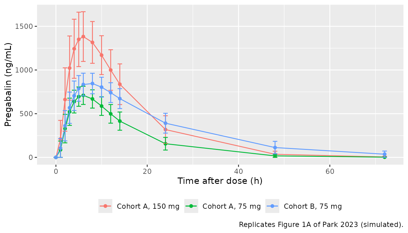
Figure 3: visual predictive check
# Replicates the simulated percentile bands of Figure 3 of Park 2023
# (10th, 50th and 90th percentiles), including residual error.
sim_tad |>
  filter(tad %in% plot_times) |>
  group_by(treatment, tad) |>
  summarise(
    p10 = quantile(sim, 0.1), p50 = quantile(sim, 0.5),
    p90 = quantile(sim, 0.9), .groups = "drop"
  ) |>
  ggplot(aes(tad)) +
  geom_ribbon(aes(ymin = p10, ymax = p90), alpha = 0.25) +
  geom_line(aes(y = p50)) +
  facet_wrap(~treatment) +
  labs(
    x = "Time after dose (h)", y = "Pregabalin (ng/mL)",
    caption = "Replicates Figure 3 of Park 2023: simulated 10th-90th percentiles and median."
  )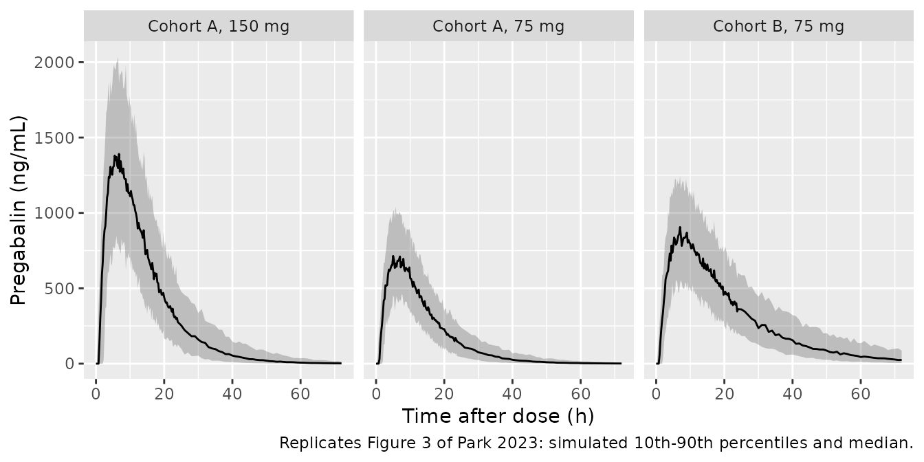
Figure 4: steady state at eGFR 90 and 45 mL/min/1.73 m^2
n_ss <- 200L
ss_scenarios <- tibble(
  scenario = c("75 mg, eGFR 90", "150 mg, eGFR 90", "75 mg, eGFR 45"),
  dose = c(75, 150, 75),
  egfr = c(90, 90, 45)
)
ss_events <- bind_rows(lapply(seq_len(nrow(ss_scenarios)), function(i) {
  ids <- (i - 1) * n_ss + seq_len(n_ss)
  doses <- tidyr::expand_grid(id = ids, time = seq(0, 13 * 24, by = 24)) |>
    mutate(amt = ss_scenarios$dose[i], evid = 1L, cmt = "depot")
  obs <- tidyr::expand_grid(id = ids, time = 312 + seq(0, 24, by = 0.5)) |>
    mutate(amt = 0, evid = 0L, cmt = "central")
  bind_rows(doses, obs) |>
    mutate(CRCL = ss_scenarios$egfr[i], OCC = 1L, scenario = ss_scenarios$scenario[i])
})) |>
  arrange(id, time, desc(evid))

sim_ss <- rxode2::rxSolve(mod, events = ss_events, keep = "scenario") |>
  as.data.frame() |>
  mutate(tad = time - 312)

ss_summary <- sim_ss |>
  group_by(scenario, tad) |>
  summarise(
    p05 = quantile(Cc, 0.05), p50 = median(Cc), p95 = quantile(Cc, 0.95),
    .groups = "drop"
  )

ggplot(ss_summary, aes(tad, colour = scenario, fill = scenario)) +
  geom_ribbon(aes(ymin = p05, ymax = p95), alpha = 0.15, colour = NA) +
  geom_line(aes(y = p50)) +
  geom_point(data = fig4_digitised, aes(time, Cc), shape = 1) +
  labs(
    x = "Time after dose at steady state (h)", y = "Pregabalin (ng/mL)",
    colour = NULL, fill = NULL,
    caption = paste(
      "Replicates Figure 4 of Park 2023. Lines: simulated median;",
      "shading: 5th-95th percentile; open circles: median digitised from the paper."
    )
  ) +
  theme(legend.position = "bottom")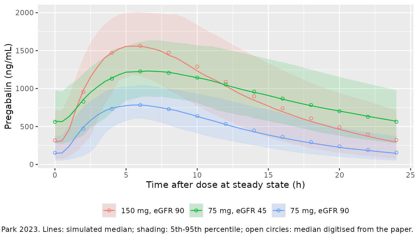
The simulated median curves reproduce the digitised ones. The median AUC over the dosing interval differs from the digitised AUC by:
auc_trap <- function(t, y) sum(diff(t) * (head(y, -1) + tail(y, -1)) / 2)
fig4_check <- ss_summary |>
  filter(tad %in% fig4_digitised$time) |>
  inner_join(fig4_digitised, by = c("scenario", tad = "time")) |>
  group_by(scenario) |>
  summarise(
    auc_simulated = auc_trap(tad, p50),
    auc_digitised = auc_trap(tad, Cc),
    .groups = "drop"
  ) |>
  mutate(pct_diff = 100 * (auc_simulated / auc_digitised - 1))

fig4_check |>
  mutate(across(c(auc_simulated, auc_digitised), round), pct_diff = round(pct_diff, 1)) |>
  rename(
    Scenario = scenario,
    "Simulated median AUC0-24 (ng*h/mL)" = auc_simulated,
    "Digitised AUC0-24 (ng*h/mL)" = auc_digitised,
    "Difference (%)" = pct_diff
  ) |>
knitr::kable()| Scenario | Simulated median AUC0-24 (ng*h/mL) | Digitised AUC0-24 (ng*h/mL) | Difference (%) |
|---|---|---|---|
| 150 mg, eGFR 90 | 21910 | 22579 | -3.0 |
| 75 mg, eGFR 45 | 22232 | 22184 | 0.2 |
| 75 mg, eGFR 90 | 11052 | 11154 | -0.9 |
PKNCA validation
NCA uses the paper’s sampling schedule. Concentrations below the 20 ng/mL lower limit of quantification are dropped after the pre-dose sample, as in the paper’s NCA.
sim_nca <- sim_tad |>
  filter(tad %in% sample_times, !is.na(Cc)) |>
  filter(tad == 0 | Cc >= 20) |>
  select(id, time = tad, Cc, treatment)

sim_nca <- bind_rows(
  sim_nca,
  sim_nca |> distinct(id, treatment) |> mutate(time = 0, Cc = 0)
) |>
  distinct(id, treatment, time, .keep_all = TRUE) |>
  arrange(id, treatment, time)

dose_df <- sim_tad |>
  distinct(id, treatment) |>
  mutate(time = 0, amt = ifelse(treatment == "Cohort A, 150 mg", 150, 75))

conc_obj <- PKNCA::PKNCAconc(sim_nca, Cc ~ time | treatment + id)
dose_obj <- PKNCA::PKNCAdose(dose_df, amt ~ time | treatment + id)
intervals <- data.frame(
  start = 0, end = Inf,
  cmax = TRUE, tmax = TRUE, auclast = TRUE, aucinf.obs = TRUE,
  half.life = TRUE, cl.obs = TRUE
)
nca_res <- PKNCA::pk.nca(PKNCA::PKNCAdata(conc_obj, dose_obj, intervals = intervals))
#> Warning: Too few points for half-life calculation (min.hl.points=3 with only 2
#> points)
Comparison against published NCA
Table 2 of Park 2023 reports arithmetic means (median for Tmax). The
simulated summaries below are aggregated the same way before comparison.
Dose is in mg and concentration in ng/mL, so PKNCA’s cl.obs
is in mg/(ng*h/mL) and is multiplied by 1000 to give L/h.
nca_long <- as.data.frame(nca_res) |>
  filter(PPTESTCD %in% c("cmax", "tmax", "auclast", "aucinf.obs", "half.life", "cl.obs")) |>
  mutate(PPORRES = ifelse(PPTESTCD == "cl.obs", 1000 * PPORRES, PPORRES))

sim_summary <- nca_long |>
  group_by(treatment, PPTESTCD) |>
  summarise(
    value = ifelse(PPTESTCD[1] == "tmax", median(PPORRES, na.rm = TRUE), mean(PPORRES, na.rm = TRUE)),
    .groups = "drop"
  ) |>
  pivot_wider(names_from = PPTESTCD, values_from = value)

published <- tibble::tribble(
  ~treatment, ~cmax, ~auclast, ~aucinf.obs, ~tmax, ~half.life, ~cl.obs,
  "Cohort A, 75 mg", 873.19, 9613.56, 10809.64, 5.0, 6.69, 7.46,
  "Cohort A, 150 mg", 1678.22, 20554.31, 22509.18, 5.0, 7.81, 7.31,
  "Cohort B, 75 mg", 1065.16, 23766.29, 25267.91, 5.5, 13.47, 3.37
)

cmp <- nlmixr2lib::ncaComparisonTable(
  simulated = sim_summary,
  reference = published,
  by = "treatment",
  units = c(
    cmax = "ng/mL", auclast = "ng*h/mL", aucinf.obs = "ng*h/mL",
    tmax = "h", half.life = "h", cl.obs = "L/h"
  ),
  tolerance_pct = 20
)
knitr::kable(
  cmp,
  caption = "Simulated vs. published (Park 2023 Table 2) NCA. * differs from reference by >20%."
)| NCA parameter | treatment | Reference | Simulated | % diff |
|---|---|---|---|---|
| Cmax (ng/mL) | Cohort A, 75 mg | 873 | 718 | -17.8% |
| Cmax (ng/mL) | Cohort A, 150 mg | 1680 | 1440 | -14.4% |
| Cmax (ng/mL) | Cohort B, 75 mg | 1070 | 857 | -19.6% |
| Tmax (h) | Cohort A, 75 mg | 5 | 6 | +20.0% |
| Tmax (h) | Cohort A, 150 mg | 5 | 6 | +20.0% |
| Tmax (h) | Cohort B, 75 mg | 5.5 | 8 | +45.5%* |
| AUC0-∞ (obs) (ng*h/mL) | Cohort A, 75 mg | 10800 | 11700 | +8.1% |
| AUC0-∞ (obs) (ng*h/mL) | Cohort A, 150 mg | 22500 | 23300 | +3.4% |
| AUC0-∞ (obs) (ng*h/mL) | Cohort B, 75 mg | 25300 | 22300 | -11.8% |
| AUClast (ng*h/mL) | Cohort A, 75 mg | 9610 | 10800 | +11.9% |
| AUClast (ng*h/mL) | Cohort A, 150 mg | 20600 | 22400 | +9.0% |
| AUClast (ng*h/mL) | Cohort B, 75 mg | 23800 | 21200 | -10.9% |
| t½ (h) | Cohort A, 75 mg | 6.69 | 6.94 | +3.7% |
| t½ (h) | Cohort A, 150 mg | 7.81 | 6.86 | -12.2% |
| t½ (h) | Cohort B, 75 mg | 13.5 | 12.9 | -4.2% |
| CL/F (L/h) | Cohort A, 75 mg | 7.46 | 6.82 | -8.6% |
| CL/F (L/h) | Cohort A, 150 mg | 7.31 | 6.85 | -6.3% |
| CL/F (L/h) | Cohort B, 75 mg | 3.37 | 3.63 | +7.7% |
AUC, half-life and CL/F agree with Table 2 to within about 12%. Simulated Cmax runs 15-20% below the observed means and Tmax is later, most visibly in Cohort B. This is a property of the published model rather than of the transcription: the typical-value one-compartment profile with ka = 0.347 1/h and V/F = 61.7 L peaks near 710 ng/mL after 75 mg at eGFR 91 mL/min/1.73 m^2, below the observed mean of 873 ng/mL, while the model’s own steady-state simulations in Figure 4 are reproduced within a few percent above. The paper notes that a structural model other than the one-compartment model “may produce a better-fitting outcome” and kept it for comparability with earlier pregabalin models.
# Table 3 of Park 2023: geometric mean ratios (Cohort B 75 mg over each
# Cohort A period) for Cmax and AUClast.
gm <- nca_long |>
  filter(PPTESTCD %in% c("cmax", "auclast")) |>
  group_by(treatment, PPTESTCD) |>
  summarise(gm = exp(mean(log(PPORRES))), .groups = "drop") |>
  pivot_wider(names_from = treatment, values_from = gm)

gmr <- tibble(
  Comparison = c("Cohort B (75 mg) / Cohort A (75 mg)", "Cohort B (75 mg) / Cohort A (150 mg)"),
  `Cmax simulated` = c(
    gm$`Cohort B, 75 mg`[gm$PPTESTCD == "cmax"] / gm$`Cohort A, 75 mg`[gm$PPTESTCD == "cmax"],
    gm$`Cohort B, 75 mg`[gm$PPTESTCD == "cmax"] / gm$`Cohort A, 150 mg`[gm$PPTESTCD == "cmax"]
  ),
  `Cmax published` = c(1.2273, 0.6476),
  `AUClast simulated` = c(
    gm$`Cohort B, 75 mg`[gm$PPTESTCD == "auclast"] / gm$`Cohort A, 75 mg`[gm$PPTESTCD == "auclast"],
    gm$`Cohort B, 75 mg`[gm$PPTESTCD == "auclast"] / gm$`Cohort A, 150 mg`[gm$PPTESTCD == "auclast"]
  ),
  `AUClast published` = c(2.4146, 1.1471)
)
knitr::kable(gmr, digits = 3, caption = "Geometric mean ratios (Park 2023 Table 3).")| Comparison | Cmax simulated | Cmax published | AUClast simulated | AUClast published |
|---|---|---|---|---|
| Cohort B (75 mg) / Cohort A (75 mg) | 1.193 | 1.227 | 1.965 | 2.415 |
| Cohort B (75 mg) / Cohort A (150 mg) | 0.596 | 0.648 | 0.945 | 1.147 |
The simulated AUClast ratio of Cohort B to Cohort A is close to 2,
which is the ratio the proportional eGFR model implies at the two cohort
medians (min(91.5, 91.2) / 45.5 = 2.0). The observed ratio
of 2.41 reflects the eight study subjects of each cohort, whose
individual eGFR values and CL/F deviations are not published.
Assumptions and deviations
- eGFR centring value (73 mL/min/1.73 m^2). Not printed in the paper; the maintainers back-solved it from the digitised median curves of Figure 4, as described above. The CL/F estimate of 5.55 L/h is therefore the typical CL/F at an eGFR of 73 mL/min/1.73 m^2.
- Breakpoint. Table 4 gives 91.2 mL/min/1.73 m^2; the Results text says the breakpoint “was fixed at the estimated value of 92.10” for the bootstrap. The model uses the tabulated final estimate, 91.2; the difference changes CL/F by at most 1% and only for eGFR above 91.2.
-
Form of the eGFR effect. The paper describes a
linear relationship through the origin (CL/F proportional to eGFR, no
separately estimated slope in Table 4) capped at the breakpoint; the
model encodes
CL/F = 5.55 * min(eGFR, 91.2) / 73. -
Inter-occasion variability. IOV on Tlag is encoded
with one eta per occasion sharing a single variance; pass
OCC = 1for single-occasion simulation. The steady-state simulation of Figure 4 uses one occasion for all doses, so its lag time varies between subjects but not between doses. - Virtual cohort. eGFR was drawn from truncated normal distributions around each cohort’s Table 1 median; individual eGFR values and their time course were not published. The study measured eGFR as a time-varying covariate, while only the screening values are reported.
- BQL data. The model was fitted with the M4 method for samples below the 20 ng/mL LLOQ. The simulation does not censor; the NCA drops post-dose simulated concentrations below 20 ng/mL to mirror the paper’s NCA.
- NCA comparison. The virtual cohorts are larger than the 8-subject study cohorts and their eGFR distribution is an approximation, so differences of the order of the published between-subject SDs are expected.
- Errata. No correction notice for this article was found in PubMed as of 2026-10-28.