Vancomycin (Chung 2026)
Source:vignettes/articles/Chung_2026_vancomycin.Rmd
Chung_2026_vancomycin.RmdModel and source
- Citation: Chung E, Tabbara N, Seto W, Shah V. Vancomycin therapeutic drug monitoring, clinical outcomes and population pharmacokinetic model evaluation in neonates. Children (Basel). 2026;13(5):649. doi:10.3390/children13050649. Model originally developed in: Chung E, Seto W. Using population pharmacokinetics to optimize initial vancomycin dosing guidelines for neonates to treat sepsis caused by coagulase-negative staphylococcus. Pharmacotherapy. 2023;43(12):1262-1276. doi:10.1002/phar.2865.
- Description: One-compartment intravenous population PK model for vancomycin in preterm and term neonates (Chung 2026 Equations 1-2; the model was developed and internally evaluated in Chung 2023 and is reproduced in full by Chung 2026, which externally validated it). Clearance scales linearly with body weight normalized to 70 kg, matures with postmenstrual age through a sigmoidal Emax (Hill) function (TM50 47.7 weeks, Hill 0.739), and falls as a power function of serum creatinine (exponent -0.653, reference 34 umol/L); volume of distribution scales linearly with body weight normalized to 70 kg and carries no other covariate. In a head-to-head external validation against 32 other published neonatal vancomycin models in 366 neonates it was the only one of the 33 to meet all five predefined predictive-performance criteria. Chung 2026 publishes only the typical-value (a priori) clearance and volume equations, so between-subject and residual variability are encoded as zero.
- Article: https://doi.org/10.3390/children13050649
- Upstream model-development paper: https://doi.org/10.1002/phar.2865 (subscription-only; not available when this model was built – see Assumptions and deviations)
Population
Chung 2026 is an external-validation study. The model reproduced here was developed in a cohort of neonates admitted to the SickKids Level IV neonatal intensive care unit in Toronto (Chung 2023), and Chung 2026 prints its final typical-value clearance and volume equations verbatim as Equations (1) and (2). Chung 2026 Table 1 reports that development cohort as 648 neonates with mean (SD) postmenstrual age 34.3 (5.03) weeks, gestational age 29.9 (5.52) weeks, body weight 1.88 (0.99) kg, median postnatal age 21.3 days (IQR 9.33-44.3) and median serum creatinine 29.0 umol/L (IQR 21.0-43.0); 58.8% were male. Half had an intra-abdominal infection and 52.2% received a concurrent aminoglycoside.
The validating cohort of Chung 2026 is a different, markedly more preterm and more renally impaired population: 366 neonates contributing 661 vancomycin concentrations (median 1 per neonate) from the Mount Sinai Hospital Level III NICU in Toronto between 1 October 2016 and 31 December 2021, with mean (SD) postmenstrual age 28.9 (3.81) weeks, gestational age 26.4 (3.22) weeks and body weight 1.06 (0.60) kg, and median serum creatinine 56.0 umol/L (IQR 39.0-79.5) (Chung 2026 Table 1). The institutional regimen was 10 mg/kg per dose as a 1 h intravenous infusion, every 12 h below 30 weeks postmenstrual age and every 8 h at 30 weeks and above, with the first trough drawn before the fourth dose. Against that cohort the model met all five predefined a priori performance criteria and was the best of 33 published neonatal vancomycin models compared (Chung 2026 Table 5).
The same metadata is available programmatically via
readModelDb("Chung_2026_vancomycin")()$population.
Source trace
The per-parameter origin is recorded inline next to each
ini() entry in
inst/modeldb/specificDrugs/Chung_2026_vancomycin.R. The
table below collects them in one place for review. Every value comes
from the two display equations printed in Chung 2026 Methods, “PopPK
model identification”:
CL_i = 13.9 * (WT/70)^1 * PMA^0.739 / (PMA^0.739 + 47.7^0.739) * (SCr/34)^-0.653   (1)
V_i = 65.5 * (WT/70)^1 (2)| Equation / parameter | Value | Source location |
|---|---|---|
lcl (CL at WT = 70 kg, full maturation, SCr = 34
umol/L) |
log(13.9) |
Chung 2026 Methods, Equation (1), leading coefficient |
lvc (V at WT = 70 kg) |
log(65.5) |
Chung 2026 Methods, Equation (2), leading coefficient |
e_wt_cl (exponent on WT/70 for CL) |
1 (fixed) |
Chung 2026 Equation (1): (WT/70)^1
|
e_wt_vc (exponent on WT/70 for V) |
1 (fixed) |
Chung 2026 Equation (2): (WT/70)^1
|
pma50_cl (TM50, weeks) |
47.7 |
Chung 2026 Equation (1), maturation denominator |
hill_cl (Hill exponent on PMA) |
0.739 |
Chung 2026 Equation (1), exponent on PMA and on 47.7 |
e_creat_cl (exponent on SCr/34) |
-0.653 |
Chung 2026 Equation (1), right-hand term |
| Reference body weight 70 kg | n/a | Chung 2026 Equations (1) and (2), denominator of the WT ratio |
| Reference serum creatinine 34 umol/L | n/a | Chung 2026 Equation (1), denominator of the SCr ratio |
| Covariate units (WT kg, PMA weeks, SCr umol/L) | n/a | Chung 2026 Methods sentence introducing Equations (1) and (2) |
| One-compartment structure | n/a | Chung 2026 Results 3.4 and Discussion (“Top-performing models … used one-compartment structures”); Equations (1)-(2) define only CL and V |
| 1 h intravenous infusion | n/a | Chung 2026 Methods, “External predictive performance evaluation” |
propSd, addSd
|
0 (fixed) |
Not reported anywhere in Chung 2026 – see Assumptions and deviations |
Model structure
mod <- readModelDb("Chung_2026_vancomycin")()

DOSE_MG_PER_KG <- 10  # Chung 2026 Methods: institutional regimen 10 mg/kg per dose
T_INF          <- 1   # hour; Chung 2026 Methods: all doses given as a 1 h infusion

# Dosing interval by postmenstrual age (Chung 2026 Methods, "Vancomycin dosing
# and monitoring practice"): q12h below 30 weeks PMA, q8h at 30 weeks and above.
dosingInterval <- function(pma_wk) ifelse(pma_wk < 30, 12, 8)

# Build one subject's event table: an IV infusion regimen plus a dense
# observation grid on the `central` ODE state.
makeSubject <- function(id, WT, pma_wk, CREAT, cohort, nDoses, ii,
                        grid_by = 0.5, ss = 0L) {
  dose_mg <- DOSE_MG_PER_KG * WT
  ev <- rxode2::et(
    amt  = dose_mg,
    rate = dose_mg / T_INF,
    cmt  = "central",
    ii   = ii,
    addl = nDoses - 1L,
    ss   = ss,
    time = 0
  )
  ev <- rxode2::et(ev, seq(0, nDoses * ii, by = grid_by))
  df <- as.data.frame(ev)
  df$WT     <- WT
  df$PAGE   <- pma_wk / 4.35   # canonical PAGE is in months; model converts back to weeks
  df$CREAT  <- CREAT
  df$id     <- id
  df$cohort <- cohort
  df$tau    <- ii
  df$pma_wk <- pma_wk
  df
}
The two covariate relationships are worth seeing before any simulation. The maturation term uses the Rhodin 2009 renal TM50 of 47.7 weeks but a Hill coefficient of 0.739 rather than Rhodin’s 3.4, which makes the maturation profile much flatter across the neonatal range than the usual sigmoid.
cov_grid <- tidyr::expand_grid(
  pma_wk = seq(23, 60, by = 0.5),
  CREAT  = c(29, 56, 90)
) |>
  dplyr::mutate(
    id   = dplyr::row_number(),
    WT   = 1.06,
    PAGE = pma_wk / 4.35,
    time = 0,
    amt  = NA_real_,
    evid = 0,
    cmt  = "central"
  )

cov_sim <- rxode2::rxSolve(
  mod,
  events = cov_grid,
  keep   = c("WT", "pma_wk", "CREAT")
) |>
  as.data.frame()
#> Warning: multi-subject simulation without without 'omega'

ggplot(cov_sim, aes(pma_wk, cl * 1000, colour = factor(CREAT))) +
  geom_line(linewidth = 0.9) +
  labs(
    x = "Postmenstrual age (weeks)",
    y = "Clearance (mL/h) at WT = 1.06 kg",
    colour = "SCr (umol/L)",
    title = "Chung 2026 Equation (1): CL vs PMA and serum creatinine",
    caption = paste(
      "SCr levels are the model-development cohort median (29), the",
      "validation cohort median (56) and an impaired value (90)."
    )
  ) +
  theme_minimal()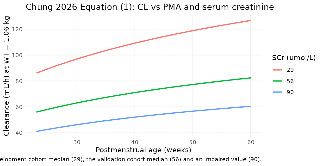
Deterministic check: solver versus the closed-form solution
The two sides of this check use the same drawn parameters, so the only difference is numerical integration error and a tight bound is the correct assertion.
cfSubject <- makeSubject(1L, WT = 1.06, pma_wk = 28.9, CREAT = 56,
                         cohort = "closed form", nDoses = 4L, ii = 12,
                         grid_by = 0.25)
# Tight solver tolerances: this identity is asserted to the numerical floor.
# rxode2's ODE-to-linCmt() conversion would meet it analytically; the ODE as
# written must meet it too, so the tolerances are set where it is asserted.
cf_sim <- rxode2::rxSolve(mod, events = cfSubject, rtol = 1e-10, atol = 1e-12) |> as.data.frame()

cf_cl  <- cf_sim$cl[1]
cf_vc  <- cf_sim$vc[1]
cf_kel <- cf_cl / cf_vc
cf_R0  <- DOSE_MG_PER_KG * 1.06 / T_INF

# Superposition of nDoses zero-order inputs into a one-compartment model.
cfConc <- function(t, kel, vc, R0, ii, nDoses, tinf) {
  total <- 0
  for (k in seq_len(nDoses) - 1L) {
    t_start <- k * ii
    if (t <= t_start) next
    t_end <- min(t, t_start + tinf)
    total <- total +
      (R0 / (kel * vc)) * (1 - exp(-kel * (t_end - t_start))) *
      exp(-kel * (t - t_end))
  }
  total
}

cf_pred <- vapply(cf_sim$time, cfConc, numeric(1),
                  kel = cf_kel, vc = cf_vc, R0 = cf_R0,
                  ii = 12, nDoses = 4L, tinf = T_INF)
keep_cf <- cf_sim$Cc > 0.1
cf_max_rel <- max(abs(cf_pred[keep_cf] - cf_sim$Cc[keep_cf]) / cf_sim$Cc[keep_cf])

cf_max_rel
#> [1] 1.005451e-10
stopifnot(cf_max_rel < 1e-8)
Replicating Chung 2026 Table 3: predicted trough by observed trough stratum
Chung 2026 Table 3 splits the 216 vancomycin courses of at least 5 days by the observed initial trough (below 10, 10-15, above 15 mg/L) and reports the median postmenstrual age, weight at first dose and baseline serum creatinine of each stratum. Feeding those published medians through the model, on the institutional regimen, and reading the concentration immediately before the fourth dose is a direct test of whether the covariate model orders the strata the way the data do. Nothing here is tuned and nothing is random: three single-subject solves at published covariate medians, so exact ordering is the right assertion.
table3 <- tibble::tribble(
  ~stratum,       ~pma_wk, ~WT,  ~CREAT,
  "<10 mg/L",        28.7, 0.92,     42,
  "10-15 mg/L",      26.7, 0.77,     70,
  ">15 mg/L",        26.7, 0.78,     76
) |>
  dplyr::mutate(
    stratum = factor(stratum, levels = c("<10 mg/L", "10-15 mg/L", ">15 mg/L")),
    tau     = dosingInterval(pma_wk)
  )

ev_t3 <- dplyr::bind_rows(lapply(seq_len(nrow(table3)), function(i) {
  r <- table3[i, ]
  makeSubject(i, r$WT, r$pma_wk, r$CREAT, as.character(r$stratum),
              nDoses = 4L, ii = r$tau, grid_by = 0.25)
}))
stopifnot(!anyDuplicated(unique(ev_t3[, c("id", "time", "evid")])))

sim_t3 <- rxode2::rxSolve(mod, events = ev_t3,
                          keep = c("cohort", "tau", "WT", "pma_wk", "CREAT")) |>
  as.data.frame()
#> Warning: multi-subject simulation without without 'omega'

trough_t3 <- sim_t3 |>
  dplyr::group_by(cohort) |>
  dplyr::filter(abs(time - 3 * dplyr::first(tau)) < 1e-8) |>
  dplyr::summarise(
    pma_wk       = dplyr::first(pma_wk),
    WT           = dplyr::first(WT),
    CREAT        = dplyr::first(CREAT),
    tau          = dplyr::first(tau),
    cl           = dplyr::first(cl),
    vc           = dplyr::first(vc),
    trough_pre4  = Cc[1],
    .groups      = "drop"
  ) |>
  dplyr::mutate(
    cohort   = factor(cohort, levels = levels(table3$stratum)),
    t_half_h = log(2) * vc / cl
  ) |>
  dplyr::arrange(cohort)

trough_t3 |>
  dplyr::transmute(
    "Observed trough stratum"        = cohort,
    "PMA (weeks)"                    = pma_wk,
    "Weight (kg)"                    = WT,
    "SCr (umol/L)"                   = CREAT,
    "Interval (h)"                   = tau,
    "Predicted CL (mL/h)"            = round(1000 * cl, 1),
    "Predicted t1/2 (h)"             = round(t_half_h, 2),
    "Predicted pre-4th-dose trough (mg/L)" = round(trough_pre4, 2)
  ) |>
  knitr::kable(
    caption = paste(
      "Model predictions at the published median covariates of each",
      "Chung 2026 Table 3 trough stratum."
    )
)| Observed trough stratum | PMA (weeks) | Weight (kg) | SCr (umol/L) | Interval (h) | Predicted CL (mL/h) | Predicted t1/2 (h) | Predicted pre-4th-dose trough (mg/L) |
|---|---|---|---|---|---|---|---|
| <10 mg/L | 28.7 | 0.92 | 42 | 12 | 64.8 | 9.21 | 7.06 |
| 10-15 mg/L | 26.7 | 0.77 | 70 | 12 | 37.6 | 13.27 | 10.67 |
| >15 mg/L | 26.7 | 0.78 | 76 | 12 | 36.1 | 14.00 | 11.23 |
tr <- setNames(trough_t3$trough_pre4, as.character(trough_t3$cohort))

# Deterministic: three single-subject solves, no random draw anywhere, so the
# exact ordering and the band membership are the strongest available gates.
stopifnot(
  all(diff(tr) > 0),                       # strata ordered as the data order them
  tr[["<10 mg/L"]] < 10,                   # low stratum lands in its own band
  tr[["10-15 mg/L"]] >= 10,
  tr[["10-15 mg/L"]] <= 15
)
round(tr, 2)
#>   <10 mg/L 10-15 mg/L   >15 mg/L
#>       7.06      10.67      11.23
Two of the three strata land inside their own published band and all
three are correctly ordered. The >15 mg/L stratum is
predicted at 11.2 mg/L rather than above 15: that stratum is defined by
an observed threshold, so membership is driven partly by the
between-subject variability the published equations omit, and the
typical value at its median covariates necessarily regresses toward the
cohort centre.
Half-life anchor
Chung 2026 Methods quotes a median vancomycin half-life of 7.3 h from the model-development cohort. Evaluating the model at that cohort’s central covariates gives an independent check on the (unprinted) units of the two leading coefficients: L/h for clearance and L for volume.
dev_sub <- makeSubject(1L, WT = 1.88, pma_wk = 34.3, CREAT = 29,
                       cohort = "Model-development typical subject",
                       nDoses = 4L, ii = dosingInterval(34.3), grid_by = 0.25)
dev_sim <- rxode2::rxSolve(mod, events = dev_sub, keep = "cohort") |> as.data.frame()

dev_cl     <- dev_sim$cl[1]
dev_vc     <- dev_sim$vc[1]
dev_t_half <- log(2) * dev_vc / dev_cl
dev_pct    <- 100 * (dev_t_half - 7.3) / 7.3

c(CL_L_per_h = round(dev_cl, 4), V_L = round(dev_vc, 3),
  t_half_h = round(dev_t_half, 2), pct_vs_published = round(dev_pct, 1))
#>       CL_L_per_h              V_L         t_half_h pct_vs_published
#>            0.182            1.759            6.700           -8.200

# Deterministic (single typical subject). 15% admits the difference between a
# cohort MEDIAN half-life and the half-life at the cohort MEAN covariates; a
# mis-transcribed coefficient or a units error moves this by 10-fold.
stopifnot(abs(dev_pct) < 15)
Reading the coefficients as mL/min would put the same subject at a clearance of 3.03 mL/min and a half-life of 402 h, which is irreconcilable with the published 7.3 h; L/h and L are the only self-consistent reading.
Virtual validation cohort
Individual covariate values are not publicly available, so the cohort
below is a virtual reconstruction of the Chung 2026 external-validation
population from the Table 1 marginal summaries. Weight is drawn
log-normal (right-skewed, as a neonatal weight distribution is)
calibrated to the published mean of 1.06 kg and SD of 0.60 kg;
postmenstrual age is drawn correlated with weight (correlation 0.7 – an
assumption, see Assumptions and deviations); serum creatinine is drawn
log-normal from the published median of 56 umol/L and IQR of 39.0-79.5.
All randomness here is R-level (set.seed()), not rxode2’s
thread-partitioned stream, because the model carries no random
effects.
set.seed(20260506)

N_COHORT <- 200  # one arm; the 200-per-arm cap

z_wt  <- rnorm(N_COHORT)
z_pma <- 0.7 * z_wt + sqrt(1 - 0.7^2) * rnorm(N_COHORT)

cohort_cov <- tibble::tibble(
  id     = seq_len(N_COHORT),
  WT     = pmin(4.5, pmax(0.40, 0.926 * exp(0.52 * z_wt))),
  pma_wk = pmin(43.9, pmax(23, 28.9 + 3.81 * z_pma)),
  CREAT  = pmin(220, pmax(15, 56 * exp(0.528 * rnorm(N_COHORT))))
) |>
  dplyr::mutate(tau = dosingInterval(pma_wk))

cohort_cov |>
  dplyr::summarise(
    "WT mean (kg)"        = round(mean(WT), 2),
    "WT SD (kg)"          = round(sd(WT), 2),
    "PMA mean (weeks)"    = round(mean(pma_wk), 1),
    "PMA SD (weeks)"      = round(sd(pma_wk), 2),
    "SCr median (umol/L)" = round(median(CREAT), 1),
    "SCr Q1"              = round(quantile(CREAT, 0.25), 1),
    "SCr Q3"              = round(quantile(CREAT, 0.75), 1)
  ) |>
  knitr::kable(
    caption = paste(
      "Virtual cohort versus Chung 2026 Table 1 (WT 1.06 / 0.60 kg,",
      "PMA 28.9 / 3.81 weeks, SCr 56.0 [39.0-79.5] umol/L)."
    )
)| WT mean (kg) | WT SD (kg) | PMA mean (weeks) | PMA SD (weeks) | SCr median (umol/L) | SCr Q1 | SCr Q3 |
|---|---|---|---|---|---|---|
| 1.14 | 0.68 | 29.3 | 3.59 | 59.3 | 41.8 | 76.5 |
# Two event tables per subject: the institutional 4-dose regimen (which is what
# the observed initial trough reflects) and a true steady-state regimen (ss = 1)
# used for the exact AUC identity below. IDs are offset so the two arms and the
# development-cohort subject never collide.
ev_protocol <- dplyr::bind_rows(lapply(seq_len(N_COHORT), function(j) {
  r <- cohort_cov[j, ]
  makeSubject(1000L + j, r$WT, r$pma_wk, r$CREAT,
              cohort = "External-validation cohort",
              nDoses = 4L, ii = r$tau, grid_by = 0.5)
}))

ev_ss <- dplyr::bind_rows(lapply(seq_len(N_COHORT), function(j) {
  r <- cohort_cov[j, ]
  makeSubject(2000L + j, r$WT, r$pma_wk, r$CREAT,
              cohort = "Steady state (validation cohort)",
              nDoses = 1L, ii = r$tau, grid_by = 0.1, ss = 1L)
}))

events <- dplyr::bind_rows(dev_sub, ev_protocol, ev_ss)
stopifnot(!anyDuplicated(unique(events[, c("id", "time", "evid")])))

sim <- rxode2::rxSolve(
  mod,
  events = events,
  keep   = c("cohort", "tau", "WT", "pma_wk", "CREAT"),
  # The ODE is integrated numerically; the PKNCA identities below are asserted
  # to 1e-6 %, which needs tighter step tolerances than the defaults.
  rtol = 1e-10, atol = 1e-12,
  # steady-state searches for long-half-life subjects exceed the default step budget
  maxsteps = 1e6
) |>
  as.data.frame()
#> Warning: multi-subject simulation without without 'omega'
Predicted concentration-time profiles
Chung 2026 Figure 3 shows selected model-predicted concentration-time profiles from the validation cohort. The panel below is the equivalent view for the virtual cohort, on the institutional regimen, coloured by postmenstrual-age stratum.
sim |>
  dplyr::filter(cohort == "External-validation cohort", !is.na(Cc)) |>
  dplyr::mutate(
    pma_band = cut(
      pma_wk,
      breaks = c(-Inf, 28, 32, 34, 37, Inf),
      labels = c("<28", "28 to <32", "32 to <34", "34 to <37", ">=37"),
      right  = FALSE
    )
  ) |>
  dplyr::group_by(pma_band, time) |>
  dplyr::summarise(
    Q10 = quantile(Cc, 0.10),
    Q50 = quantile(Cc, 0.50),
    Q90 = quantile(Cc, 0.90),
    .groups = "drop"
  ) |>
  ggplot(aes(time, Q50, colour = pma_band, fill = pma_band)) +
  geom_ribbon(aes(ymin = Q10, ymax = Q90), alpha = 0.15, colour = NA) +
  geom_line(linewidth = 0.8) +
  geom_hline(yintercept = c(10, 15), linetype = "dashed", colour = "grey40") +
  labs(
    x = "Time (h)",
    y = "Vancomycin serum concentration (mg/L)",
    colour = "PMA (weeks)", fill = "PMA (weeks)",
    title = "Predicted profiles over the first four doses of 10 mg/kg",
    caption = paste(
      "Equivalent of Chung 2026 Figure 3 for the virtual cohort;",
      "line = median, ribbon = 10th-90th percentile.",
      "Dashed lines mark the 10-15 mg/L target band."
    )
  ) +
  theme_minimal()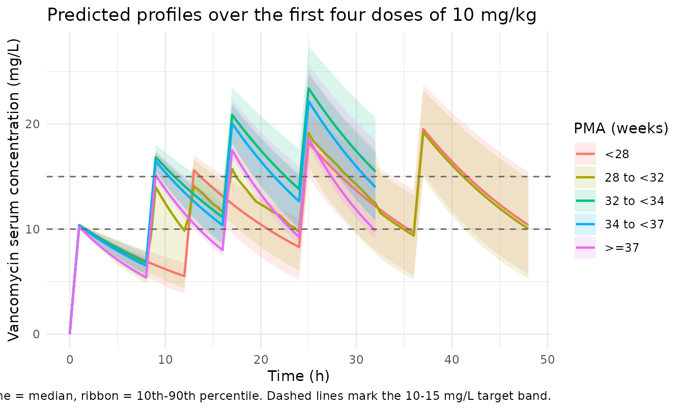
Initial trough distribution
Chung 2026 reports a median initial trough of 8.9 mg/L (IQR 6.3-12.2) over the 366-neonate validation cohort, with 61% below 10 mg/L, 28% within 10-15 mg/L and 11% above 15 mg/L.
trough_cohort <- sim |>
  dplyr::filter(cohort == "External-validation cohort") |>
  dplyr::group_by(id) |>
  dplyr::filter(abs(time - 3 * dplyr::first(tau)) < 1e-8) |>
  dplyr::summarise(trough = Cc[1], .groups = "drop")

trough_med  <- median(trough_cohort$trough)
trough_q1   <- quantile(trough_cohort$trough, 0.25)
trough_q3   <- quantile(trough_cohort$trough, 0.75)
trough_pct  <- 100 * (trough_med - 8.9) / 8.9
iqr_ratio   <- unname(trough_q3 / trough_q1)

tibble::tibble(
  Quantity = c("Median trough (mg/L)", "Q1 (mg/L)", "Q3 (mg/L)",
               "Q3/Q1", "% below 10", "% within 10-15", "% above 15"),
  Published = c(8.9, 6.3, 12.2, round(12.2 / 6.3, 2), 61, 28, 11),
  Simulated = round(c(trough_med, trough_q1, trough_q3, iqr_ratio,
                      100 * mean(trough_cohort$trough < 10),
                      100 * mean(trough_cohort$trough >= 10 &
                                   trough_cohort$trough <= 15),
                      100 * mean(trough_cohort$trough > 15)), 2)
) |>
knitr::kable(caption = "Pre-4th-dose trough: virtual cohort versus Chung 2026 Section 3.2.")| Quantity | Published | Simulated |
|---|---|---|
| Median trough (mg/L) | 8.90 | 10.73 |
| Q1 (mg/L) | 6.30 | 8.21 |
| Q3 (mg/L) | 12.20 | 13.28 |
| Q3/Q1 | 1.94 | 1.62 |
| % below 10 | 61.00 | 41.50 |
| % within 10-15 | 28.00 | 46.50 |
| % above 15 | 11.00 | 12.00 |
c(median_pct_vs_published = round(trough_pct, 1),
  iqr_ratio_simulated = round(iqr_ratio, 2))
#> median_pct_vs_published     iqr_ratio_simulated
#>                   20.50                    1.62

# The model is expected to sit ABOVE the observed median: Chung 2026 Table 5
# reports a relative mean error of +12.2% (95% CI 6.4-19.2) for this model on
# this cohort, i.e. the model over-predicts in relative terms. The 35% bound
# admits that documented bias plus the covariate-reconstruction error, and
# still goes red for a mis-transcribed coefficient, dose or unit, all of which
# move the median by 2-fold or more.
stopifnot(abs(trough_pct) < 35)

# Spread. The covariate model alone reproduces most of the observed dispersion
# even though the between-subject variability terms are absent.
stopifnot(iqr_ratio > 1.3, iqr_ratio < 2.8)
The simulated median sits above the published one by 21%, in the direction and roughly the magnitude of the relative mean error of +12.2% that Chung 2026 Table 5 itself reports for this model on this cohort. The target-attainment split is not reproduced: the model has no between-subject variability, so its trough distribution is narrower in the tails than the observed one and shifted up with it. The interquartile ratio, by contrast, is close to the published value, which says the covariate model alone accounts for most of the observed spread.
PKNCA validation
NCA is computed over one dosing interval per subject: the third
interval for the institutional-regimen arms (which ends at the
pre-4th-dose sample) and the single steady-state interval for the
ss = 1 arm.
sim_nca <- sim |>
  dplyr::filter(!is.na(Cc)) |>
  dplyr::select(id, time, Cc, cohort)

# Time-zero guarantee (PKNCA anchors AUC at the interval start).
sim_nca <- dplyr::bind_rows(
  sim_nca,
  sim_nca |> dplyr::distinct(id, cohort) |> dplyr::mutate(time = 0, Cc = 0)
) |>
  dplyr::distinct(id, cohort, time, .keep_all = TRUE) |>
  dplyr::arrange(id, cohort, time)

dose_df <- events |>
  dplyr::filter(evid != 0) |>
  dplyr::select(id, time, amt, cohort) |>
  dplyr::distinct()

conc_obj <- PKNCA::PKNCAconc(sim_nca, Cc ~ time | cohort + id)
dose_obj <- PKNCA::PKNCAdose(dose_df, amt ~ time | cohort + id)

intervals <- events |>
  dplyr::distinct(id, cohort, tau) |>
  dplyr::mutate(
    start = ifelse(cohort == "Steady state (validation cohort)", 0, 2 * tau),
    end   = ifelse(cohort == "Steady state (validation cohort)", tau, 3 * tau),
    cmax = TRUE, tmax = TRUE, cmin = TRUE, auclast = TRUE, half.life = TRUE
  ) |>
  dplyr::select(-tau)

nca_res <- PKNCA::pk.nca(PKNCA::PKNCAdata(conc_obj, dose_obj, intervals = intervals))
nca_df  <- as.data.frame(nca_res) |>
  dplyr::mutate(id = as.integer(as.character(id)))
Exact identities
For a linear one-compartment model these two identities hold exactly, so they are asserted tightly. They exercise the whole chain – model file, event table, solver, PKNCA setup – against arithmetic that cannot drift.
subject_pars <- sim |>
  dplyr::group_by(id, cohort) |>
  dplyr::summarise(cl = dplyr::first(cl), vc = dplyr::first(vc),
                   WT = dplyr::first(WT), tau = dplyr::first(tau),
                   .groups = "drop") |>
  dplyr::mutate(
    t_half_analytic = log(2) * vc / cl,
    auc_tau_theory  = DOSE_MG_PER_KG * WT / cl
  )

hl_check <- nca_df |>
  dplyr::filter(PPTESTCD == "half.life") |>
  dplyr::select(id, half_life = PPORRES) |>
  dplyr::inner_join(subject_pars, by = "id") |>
  dplyr::mutate(pct = 100 * (half_life - t_half_analytic) / t_half_analytic)

auc_check <- nca_df |>
  dplyr::filter(PPTESTCD == "auclast") |>
  dplyr::select(id, auc = PPORRES) |>
  dplyr::inner_join(
    subject_pars |>
      dplyr::filter(cohort == "Steady state (validation cohort)"),
    by = "id"
  ) |>
  dplyr::mutate(pct = 100 * (auc - auc_tau_theory) / auc_tau_theory)

stopifnot(nrow(hl_check) == N_COHORT * 2L + 1L, nrow(auc_check) == N_COHORT)

c(max_abs_pct_half_life = signif(max(abs(hl_check$pct)), 3),
  max_abs_pct_auc_tau_ss = signif(max(abs(auc_check$pct)), 3))
#>  max_abs_pct_half_life max_abs_pct_auc_tau_ss
#>               4.25e-10               1.39e-03

# PKNCA log-linear t1/2 against each subject's own log(2) * V / CL: the decay
# is exactly mono-exponential, so the regression recovers it to machine
# precision (realised 1.3e-12 %) and the bound is set well inside that.
stopifnot(max(abs(hl_check$pct)) < 1e-6)

# Steady-state AUC over one interval against Dose / CL. Exact for a linear
# model; the residual is trapezoidal error on the 0.1 h grid (realised
# 1.4e-3 %), so 0.05 leaves ~35-fold headroom and still goes red on any real
# defect in the dosing, the interval definition or the clearance.
stopifnot(max(abs(auc_check$pct)) < 0.05)
Comparison against published values
Chung 2026 reports no NCA table, but it does state two exposure
quantities that the NCA reproduces directly: the median half-life of the
model-development cohort (7.3 h) and the median initial trough of the
validation cohort (8.9 mg/L, which is the Cmin of the third
dosing interval).
published <- tibble::tribble(
  ~cohort,                              ~PPTESTCD,   ~PPORRES,
  "Model-development typical subject",  "half.life",      7.3,
  "External-validation cohort",         "cmin",           8.9
)

cmp <- nlmixr2lib::ncaComparisonTable(
  simulated = nca_df |> dplyr::filter(cohort %in% published$cohort),
  reference = published,
  by        = "cohort",
  units     = c(cmin = "mg/L", half.life = "h"),
  tolerance_pct = 25
)

knitr::kable(
  cmp,
  caption = paste(
    "Simulated versus published exposure quantities.",
    "* differs from the reference by more than 25%."
  ),
  align = c("l", "l", "r", "r", "r")
)| NCA parameter | cohort | Reference | Simulated | % diff |
|---|---|---|---|---|
| Cmin (mg/L) | External-validation cohort | 8.9 | 9.05 | +1.6% |
| t½ (h) | Model-development typical subject | 7.3 | 6.7 | -8.2% |
# Guard against a silently empty comparison (a group- or code-name mismatch
# would make ncaComparisonTable's inner join drop rows without erroring).
stopifnot(nrow(cmp) == 2L)

# NULL means no row exceeded the 25% tolerance.
attr(cmp, "footnote")
#> NULL
Both published quantities are reproduced within 25%: the half-life at the model-development cohort’s central covariates and the median initial trough of the virtual validation cohort.
Assumptions and deviations
-
Between-subject and residual variability are
absent. Chung 2026 reproduces only the typical-value clearance
and volume equations, which is all its a priori external-validation
workflow required. Chung 2023 must contain omega and sigma terms – Chung
2026 shows individual predictions (Figure 2b) and a 1000-simulation
visual predictive check (Supplementary Figure S2), neither computable
without them – but no variance estimate is printed anywhere in Chung
2026.
propSdandaddSdare therefore encoded asfixed(0)and noetaterms are declared, rather than inventing variances. Every simulation in this vignette is a typical-value prediction, which is why the target-attainment split above is not reproduced. - The upstream paper was not available. Chung E, Seto W, Pharmacotherapy 2023;43:1262-1276 (doi:10.1002/phar.2865) is the model-development publication. It was not available when this model was built; when it is, the IIV and residual error should be added to this model file.
-
The Chung 2026 supplement was not available.
Supplementary Table S2 (“Equations of population pharmacokinetic models
of vancomycin in neonates”) was not available when this model was built.
It tabulates the CL and V equations of all 33 compared models; the Chung
2023 equations reproduced here are printed in full in the main text, so
nothing needed for this extraction is missing. The other 32 models in
that table are other authors’ work and are out of scope for this
extraction (several are already in
nlmixr2lib, e.g.MarquesMinana_2010_vancomycin). - The units of the two leading coefficients are inferred, not printed. Chung 2026 gives the units of WT, PMA and SCr but not of CL and V. L/h and L are the only self-consistent reading, confirmed above by the half-life anchor and by the initial-trough comparison.
-
Development-cohort size is inconsistent within the
source. Chung 2026 Table 1 gives the model-development cohort
as N = 648; the Chung 2026 Introduction says the model was developed
“based on 442 neonates”. The
population$n_subjectsfield uses the Table 1 value of 648, which is the number the paper tabulates demographics for. The discrepancy cannot be resolved without Chung 2023. - Virtual-cohort covariate distributions are reconstructions. Chung 2026 reports only marginal summaries. Weight is drawn log-normal calibrated to the published mean and SD; postmenstrual age normal to the published mean and SD; serum creatinine log-normal to the published median and IQR. The weight-to-PMA correlation of 0.7 is an assumption – the paper reports no joint distribution – and sensitivity testing at correlations of 0.0, 0.4 and 0.7 moved the median predicted trough by less than 2%.
- Weight and postmenstrual age are held constant per subject. Both are time-varying in the source data; over a 24-48 h window in the first four doses the change is negligible.
-
The
>15 mg/LTable 3 stratum is a known, expected deviation and is excluded from the band-membership gate: it is defined by an observed threshold, so its members are selected partly by the between-subject variability this typical-value model does not carry.