Baloxavir (Koshimichi 2020)
Source:vignettes/articles/Koshimichi_2020_baloxavir.Rmd
Koshimichi_2020_baloxavir.RmdModel and source
- Citation: Koshimichi H, Retout S, Cosson V, Duval V, De Buck S, Tsuda Y, Ishibashi T, Wajima T. Population Pharmacokinetics and Exposure-Response Relationships of Baloxavir Marboxil in Influenza Patients at High Risk of Complications. Antimicrob Agents Chemother. 2020;64(7):e00119-20. doi:10.1128/AAC.00119-20
- Description: Three-compartment population PK model with first-order absorption and an absorption lag time for baloxavir acid (the active form of the prodrug baloxavir marboxil) in healthy adults and in otherwise healthy and high-risk adult and adolescent influenza patients, with bodyweight, race (Asian vs non-Asian) and sex covariates (Koshimichi 2020)
- Article (open access): https://doi.org/10.1128/AAC.00119-20
- Supplement (Tables S1-S3, Figures S1-S10): supplemental file 1 of the article.
Baloxavir marboxil is an oral prodrug of baloxavir acid, an inhibitor of the influenza cap-dependent endonuclease. Koshimichi 2020 pooled 13 clinical studies - ten phase 1 studies in healthy subjects, a phase 2 and a phase 3 (CAPSTONE-1) study in otherwise healthy influenza patients, and the phase 3 CAPSTONE-2 study in patients at high risk of influenza complications - to develop a population PK model of baloxavir acid, and then related the individual exposures to the time to improvement of influenza symptoms and to the day-2 virus-titer reduction in the high-risk patients.
The packaged model is the final model (model no. 523) of Koshimichi 2020 Table 2: a three-compartment disposition model with first-order absorption and an absorption lag time; power bodyweight effects with one exponent shared by the three clearances and a second shared by the three volumes; multiplicative race (Asian vs non-Asian) effects on CL/F and Vc/F; and a sex effect on ka.
The exposure-response part of the paper is descriptive only (median TTIIS and virus-titer change per exposure category, Tables 4 and 5); no exposure-response model was fitted, so there is no PD model to package.
Doses are baloxavir marboxil doses in mg and concentrations are baloxavir acid concentrations in ng/mL, as in the paper.
Population
The analysis dataset held 11,846 baloxavir acid plasma concentrations from 1,827 subjects (Koshimichi 2020 Results; Table S1, Table S2f): 277 healthy subjects (231 Asian, 46 non-Asian) and 1,550 influenza patients (844 Asian, 706 non-Asian), of whom 664 were CAPSTONE-2 patients at high risk of influenza complications. Healthy subjects were 20-70 years old and patients 12-85 years; bodyweight ranged from 36.0 to 217.3 kg; 809 subjects (44.3%) were female (Table 1). Phase 3 patients received a single 40 mg dose (40 to <80 kg) or 80 mg dose (>=80 kg).
str(readModelDb("Koshimichi_2020_baloxavir")()$population)
#> List of 13
#>  $ species       : chr "human"
#>  $ n_subjects    : num 1827
#>  $ n_studies     : num 13
#>  $ n_observations: num 11846
#>  $ age_range     : chr "12-85 years"
#>  $ weight_range  : chr "36.0-217.3 kg"
#>  $ weight_median : chr "67.7 kg (reference weight of the covariate model)"
#>  $ sex_female_pct: num 44.3
#>  $ race_ethnicity: Named num [1:2] 58.8 41.2
#>   ..- attr(*, "names")= chr [1:2] "Asian" "Non-Asian"
#>  $ disease_state : chr "277 healthy subjects from 10 phase 1 studies; 1,550 influenza patients from a phase 2 and a phase 3 study in ot"| __truncated__
#>  $ dose_range    : chr "Single oral doses of baloxavir marboxil 6-80 mg; 40 mg (<80 kg) or 80 mg (>=80 kg) in the phase 3 studies"
#>  $ regions       : chr "Japan, United States, United Kingdom and global phase 3 sites"
#>  $ notes         : chr "Pooled from 13 clinical studies (Koshimichi 2020 Table S1). Baseline demographics by health status and race in "| __truncated__
Source trace
Every ini() value carries an in-file comment in
inst/modeldb/specificDrugs/Koshimichi_2020_baloxavir.R; the
table collects them in one place.
| Equation / parameter | Value | Source location |
|---|---|---|
lcl (CL/F) |
10.8 L/h | Table 2 (RSE 1.8%) |
lvc (Vc/F) |
565 L | Table 2 (RSE 3.0%) |
lq (Q1/F) |
12.4 L/h | Table 2 (RSE 6.9%) |
lvp (Vp1/F) |
141 L | Table 2 (RSE 3.1%) |
lq2 (Q2/F) |
1.43 L/h | Table 2 (RSE 4.3%) |
lvp2 (Vp2/F) |
139 L | Table 2 (RSE 2.4%) |
lka (Ka) |
1.03 1/h | Table 2 (RSE 6.3%); unit printed as “liters/h”, 1/h per the footnote equation |
ltlag (lag time) |
0.345 h | Table 2 (RSE 3.3%) |
e_wt_cl_q |
0.362 | Table 2, effect of body wt on CL/F, Q1/F, Q2/F |
e_wt_vc_vp |
0.833 | Table 2, effect of body wt on Vc/F, Vp1/F, Vp2/F |
e_race_asian_cl |
0.519 | Table 2, effect of race (Asian) on CL/F |
e_race_asian_vc |
0.564 | Table 2, effect of race (Asian) on Vc/F |
e_sexf_ka |
0.682 | Table 2, effect of gender on Ka |
| IIV CL/F, Vc/F | CV 41.1%, 62.7% -> omega^2 0.1689, 0.3931 | Table 2; see Assumptions for the scale |
| CL/F-Vc/F covariance | 0.209 | Table 2 |
| IIV Vp1/F, Vp2/F, Ka | CV 29.3%, 35.4%, 123.7% | Table 2 |
propSd |
0.202 | Table 2, proportional residual error 20.2% |
| Covariate equations, reference weight 67.7 kg, Asian / gender coding | n/a | Table 2 footnote; Figure S1 legend |
| Three-compartment, first-order absorption with lag structure | n/a | Results, first paragraph; Table S2a |
| No IIV on Q1/F, Q2/F or lag time; proportional-only residual error | n/a | Table S2a model 011, Table S2c models 206-210; parameter count 20 for model 523 (Table S2f) |
Structural checks (typical values)
For a linear model the AUC0-inf of a single dose equals
1000 * dose / (CL/F) (mg / (L/h) scaled to ng*h/mL). Both
sides use the same typical-value parameters, so the bound is tight.
mod <- readModelDb("Koshimichi_2020_baloxavir")
mod_typical <- rxode2::zeroRe(mod)
#> ℹ parameter labels from comments will be replaced by 'label()'

typ_design <- tidyr::expand_grid(
  WT = c(55, 67.7, 90), RACE_ASIAN = c(0, 1), SEXF = c(0, 1)
) |>
  dplyr::mutate(id = dplyr::row_number(), dose = ifelse(WT >= 80, 80, 40))

obs_times <- sort(unique(c(seq(0, 12, by = 0.1), seq(12, 48, by = 1),
                           seq(48, 3000, by = 12))))

typ_events <- dplyr::bind_rows(
  typ_design |> dplyr::transmute(id, time = 0, amt = dose, evid = 1L, cmt = "depot"),
  typ_design |> dplyr::select(id) |> tidyr::expand_grid(time = obs_times) |>
    dplyr::mutate(amt = NA_real_, evid = 0L, cmt = "central")
) |>
  dplyr::left_join(typ_design |> dplyr::select(id, WT, RACE_ASIAN, SEXF), by = "id") |>
  dplyr::arrange(id, time, dplyr::desc(evid))

typ_sim <- rxode2::rxSolve(mod_typical, typ_events, returnType = "data.frame")
#> ℹ omega/sigma items treated as zero: 'etalcl', 'etalvc', 'etalvp', 'etalvp2', 'etalka'
#> Warning: multi-subject simulation without without 'omega'

auc_check <- typ_sim |>
  dplyr::group_by(id) |>
  dplyr::summarise(
    cl = dplyr::first(cl),
    auc_last = sum(diff(time) * (utils::head(Cc, -1) + utils::tail(Cc, -1)) / 2),
    lz = -diff(log(Cc[c(dplyr::n() - 20L, dplyr::n())])) /
      diff(time[c(dplyr::n() - 20L, dplyr::n())]),
    c_last = dplyr::last(Cc),
    .groups = "drop"
  ) |>
  dplyr::left_join(typ_design, by = "id") |>
  dplyr::mutate(
    auc_sim = auc_last + c_last / lz,
    auc_exact = 1000 * dose / cl,
    pct_diff = 100 * (auc_sim - auc_exact) / auc_exact
  )
stopifnot(max(abs(auc_check$pct_diff)) < 0.5)

# Covariate identities: race ratio on CL/F and allometric ratio.
cl_of <- function(wt, asian) {
  unique(auc_check$cl[auc_check$WT == wt & auc_check$RACE_ASIAN == asian])
}
stopifnot(
  abs(cl_of(67.7, 1) / cl_of(67.7, 0) - 0.519) < 1e-8,
  abs(cl_of(67.7, 0) - 10.8) < 1e-8,
  abs(cl_of(90, 0) / cl_of(55, 0) - (90 / 55)^0.362) < 1e-8
)
summary(auc_check$pct_diff)
#>    Min. 1st Qu.  Median    Mean 3rd Qu.    Max.
#> 0.07912 0.09293 0.10716 0.10953 0.12799 0.14301
typ_sim |>
  dplyr::left_join(typ_design, by = c("id", "WT", "RACE_ASIAN", "SEXF")) |>
  dplyr::filter(SEXF == 0, time <= 240, time > 0) |>
  dplyr::mutate(
    group = paste0(WT, " kg, ", dose, " mg"),
    race = ifelse(RACE_ASIAN == 1, "Asian", "non-Asian")
  ) |>
  ggplot(aes(time, Cc, colour = group, linetype = race)) +
  geom_line() +
  scale_y_log10() +
  labs(x = "Time after dose (h)", y = "Baloxavir acid (ng/mL)",
       colour = NULL, linetype = NULL)
#> Warning in scale_y_log10(): log-10 transformation introduced infinite values.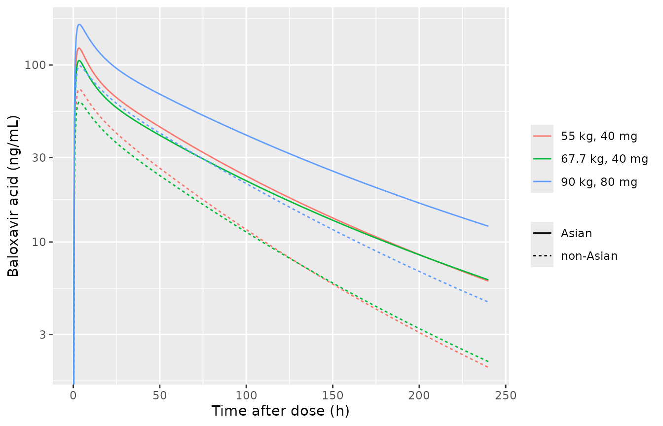
Typical-value baloxavir acid profiles after a single 40 mg (55 and 67.7 kg) or 80 mg (90 kg) dose of baloxavir marboxil, males.
Virtual cohort: phase 3 high-risk patients
Table 3 summarises the individual exposures by dose (bodyweight group) and race for the phase 3 studies. The virtual cohort mimics the CAPSTONE-2 arms: four groups (40 mg for 40 to <80 kg, 80 mg for >=80 kg; Asian and non-Asian) of 200 patients each. Bodyweight is drawn from a log-normal distribution with the median and SD of the Table 1 patient columns for that race (Asian median 61.9 kg, SD 13.5; non-Asian median 80.0 kg, SD 21.7), truncated to the dose group’s weight band. The female fraction follows Table 1 (Asian patients 42.3%, non-Asian patients 59.3%).
rxode2::rxSetSeed(20200623)
set.seed(20200623)
n_per_arm <- 200

draw_wt <- function(n, median_wt, mean_wt, sd_wt, lo, hi) {
  sdlog <- sqrt(log(1 + (sd_wt / mean_wt)^2))
  u <- stats::runif(n, stats::plnorm(lo, log(median_wt), sdlog),
                    stats::plnorm(hi, log(median_wt), sdlog))
  stats::qlnorm(u, log(median_wt), sdlog)
}

arms <- tibble::tribble(
  ~arm,                          ~asian, ~dose, ~lo, ~hi,   ~med, ~mean, ~sd,  ~pfem,
  "40 mg (<80 kg), Asian",           1,    40,  40,   80,  61.9,  63.4, 13.5, 0.423,
  "40 mg (<80 kg), non-Asian",       0,    40,  40,   80,  80.0,  83.1, 21.7, 0.593,
  "80 mg (>=80 kg), Asian",          1,    80,  80,  150,  61.9,  63.4, 13.5, 0.423,
  "80 mg (>=80 kg), non-Asian",      0,    80,  80,  217,  80.0,  83.1, 21.7, 0.593
)

cohort <- arms |>
  dplyr::rowwise() |>
  dplyr::reframe(
    arm = arm, RACE_ASIAN = asian, dose = dose,
    WT = draw_wt(n_per_arm, med, mean, sd, lo, hi),
    SEXF = stats::rbinom(n_per_arm, 1, pfem)
  ) |>
  dplyr::mutate(id = dplyr::row_number())

sim_times <- sort(unique(c(seq(0, 12, by = 0.25), seq(12, 48, by = 2), 24,
                           seq(48, 720, by = 24))))

events <- dplyr::bind_rows(
  cohort |> dplyr::transmute(id, time = 0, amt = dose, evid = 1L, cmt = "depot"),
  cohort |> dplyr::select(id) |> tidyr::expand_grid(time = sim_times) |>
    dplyr::mutate(amt = NA_real_, evid = 0L, cmt = "central")
) |>
  dplyr::left_join(cohort |> dplyr::select(id, arm, WT, RACE_ASIAN, SEXF), by = "id") |>
  dplyr::arrange(id, time, dplyr::desc(evid))

sim <- rxode2::rxSolve(mod, events, keep = "arm", returnType = "data.frame") |>
  dplyr::mutate(arm = as.character(arm))
#> ℹ parameter labels from comments will be replaced by 'label()'
Concentration-time profiles
sim |>
  dplyr::filter(time > 0, time <= 240) |>
  dplyr::group_by(arm, time) |>
  dplyr::summarise(
    med = stats::median(Cc), lo = stats::quantile(Cc, 0.025),
    hi = stats::quantile(Cc, 0.975), .groups = "drop"
  ) |>
  ggplot(aes(time, med)) +
  geom_ribbon(aes(ymin = lo, ymax = hi), fill = "grey80") +
  geom_line() +
  facet_wrap(~arm) +
  scale_y_log10() +
  labs(x = "Time after dose (h)", y = "Baloxavir acid (ng/mL)")
#> Warning in scale_y_log10(): log-10 transformation introduced infinite values.
#> log-10 transformation introduced infinite values.
#> log-10 transformation introduced infinite values.
#> log-10 transformation introduced infinite values.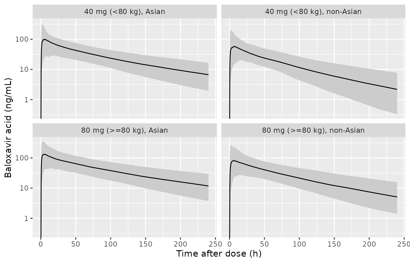
Simulated median and 95% prediction interval of baloxavir acid concentrations (individual predictions, residual error excluded) in the virtual high-risk patient arms; compare with the Phase 2/3 panels of Koshimichi 2020 Figure 1.
PKNCA
sim_nca <- sim |>
  dplyr::filter(!is.na(Cc)) |>
  dplyr::select(id, time, Cc, arm)
sim_nca <- dplyr::bind_rows(
  sim_nca,
  sim_nca |> dplyr::distinct(id, arm) |> dplyr::mutate(time = 0, Cc = 0)
) |>
  dplyr::distinct(id, arm, time, .keep_all = TRUE) |>
  dplyr::arrange(id, arm, time)

conc_obj <- PKNCA::PKNCAconc(sim_nca, Cc ~ time | arm + id)
dose_obj <- PKNCA::PKNCAdose(
  events |> dplyr::filter(evid == 1) |> dplyr::select(id, time, amt, arm),
  amt ~ time | arm + id
)
intervals <- data.frame(start = 0, end = Inf, cmax = TRUE, tmax = TRUE,
                        aucinf.obs = TRUE, half.life = TRUE)
nca_res <- PKNCA::pk.nca(PKNCA::PKNCAdata(conc_obj, dose_obj, intervals = intervals))

# C24 is a spot concentration, not an interval NCA parameter; it is appended
# with the carrier code "ctrough" and relabelled in the comparison table.
c24 <- sim |>
  dplyr::filter(abs(time - 24) < 1e-6) |>
  dplyr::transmute(arm, id, PPTESTCD = "ctrough", PPORRES = Cc)

sim_long <- dplyr::bind_rows(
  as.data.frame(nca_res$result) |> dplyr::select(arm, id, PPTESTCD, PPORRES),
  c24
)
Comparison against Table 3 (high-risk patients)
published <- tibble::tribble(
  ~arm,                          ~cmax, ~aucinf.obs, ~ctrough,
  "40 mg (<80 kg), Asian",         104,        6380,     64.0,
  "40 mg (<80 kg), non-Asian",    60.6,        3661,     35.9,
  "80 mg (>=80 kg), Asian",        137,        9733,     87.6,
  "80 mg (>=80 kg), non-Asian",   84.9,        5737,     58.7
)

cmp <- nlmixr2lib::ncaComparisonTable(
  simulated = sim_long,
  reference = published,
  by = "arm",
  params = c("cmax", "aucinf.obs", "ctrough"),
  units = c(cmax = "ng/mL", aucinf.obs = "ng*h/mL", ctrough = "ng/mL"),
  tolerance_pct = 20
)
cmp[["NCA parameter"]] <- sub("^Ctrough ", "C24 ", cmp[["NCA parameter"]])
knitr::kable(
  cmp,
  caption = paste(
    "Simulated medians vs the medians of Koshimichi 2020 Table 3",
    "(phase 3 patients at high risk of influenza complications).",
    attr(cmp, "footnote")
  )
)| NCA parameter | arm | Reference | Simulated | % diff |
|---|---|---|---|---|
| Cmax (ng/mL) | 40 mg (<80 kg), Asian | 104 | 109 | +4.9% |
| Cmax (ng/mL) | 40 mg (<80 kg), non-Asian | 60.6 | 62.7 | +3.5% |
| Cmax (ng/mL) | 80 mg (>=80 kg), Asian | 137 | 141 | +3.0% |
| Cmax (ng/mL) | 80 mg (>=80 kg), non-Asian | 84.9 | 85.3 | +0.5% |
| AUC0-∞ (obs) (ng*h/mL) | 40 mg (<80 kg), Asian | 6380 | 7660 | +20.0%* |
| AUC0-∞ (obs) (ng*h/mL) | 40 mg (<80 kg), non-Asian | 3660 | 3850 | +5.2% |
| AUC0-∞ (obs) (ng*h/mL) | 80 mg (>=80 kg), Asian | 9730 | 12000 | +23.5%* |
| AUC0-∞ (obs) (ng*h/mL) | 80 mg (>=80 kg), non-Asian | 5740 | 6750 | +17.7% |
| C24 (ng/mL) | 40 mg (<80 kg), Asian | 64 | 63.2 | -1.3% |
| C24 (ng/mL) | 40 mg (<80 kg), non-Asian | 35.9 | 38.6 | +7.5% |
| C24 (ng/mL) | 80 mg (>=80 kg), Asian | 87.6 | 89.2 | +1.8% |
| C24 (ng/mL) | 80 mg (>=80 kg), non-Asian | 58.7 | 60 | +2.2% |
pct <- sim_long |>
  dplyr::filter(PPTESTCD %in% c("cmax", "aucinf.obs", "ctrough")) |>
  dplyr::group_by(arm, PPTESTCD) |>
  dplyr::summarise(sim = stats::median(PPORRES), .groups = "drop") |>
  dplyr::inner_join(
    published |> tidyr::pivot_longer(-arm, names_to = "PPTESTCD", values_to = "ref"),
    by = c("arm", "PPTESTCD")
  ) |>
  dplyr::mutate(pct_diff = 100 * (sim - ref) / ref)
stopifnot(nrow(pct) == 12L)
stopifnot(
  abs(stats::median(pct$pct_diff)) < 15,
  stats::quantile(abs(pct$pct_diff), 0.9) < 30
)
Cmax and C24 reproduce the published medians to within about 8% in all four arms, including the roughly two-fold Asian vs non-Asian exposure difference. The simulated AUC0-inf runs high by about 5% in the 40 mg non-Asian arm and by about 18-24% in the other three arms, with the largest gaps in the two Asian arms, which have the lowest CL/F and hence the longest terminal phase. Table 3 does not state the AUC interval; a published AUC truncated to a finite interval, or extrapolated per individual from sparse phase 3 samples, would fall short of the model’s full AUC0-inf in this direction (the shortfall grows as CL/F falls). The arm bodyweights are also only approximated (see Assumptions), and bodyweight moves AUC through CL/F. Cmax and C24, the two metrics with an unambiguous definition, are the stronger check. No parameter was adjusted.
Assumptions and deviations
- IIV scale. Table 2 prints each IIV as “% CV” but the CL/F-Vc/F covariance as a raw value (0.209). A covariance can only be reported on the raw OMEGA scale, so the diagonals are taken on the same scale: omega^2 = (CV/100)^2. The printed %RSEs support this: the bootstrap 95% CIs of the CL/F, Vc/F and Ka rows imply omega^2 RSEs of 4.5%, 4.6% and 7.1% under this reading (printed 4.4%, 4.6% and 6.9%), versus 4.1%, 3.9% and 4.6% under the omega^2 = log(1 + CV^2) reading. The resulting CL/F-Vc/F correlation is 0.81.
- Ka unit. Table 2 prints the Ka unit as “liters/h”; it is a first-order rate constant (1/h), as in the Table 2 footnote equation.
- Dose basis. No molecular-weight correction between baloxavir marboxil and baloxavir acid appears in the paper; CL/F and V/F are taken as referenced to the administered baloxavir marboxil dose, as in the prior baloxavir models.
-
Removed covariates. ALT on CL/F, age on CL/F and
Vc/F, gender on Vc/F and food (fed) on F were in the full model but
removed from the final model; they are documented in
covariatesDataExcludedand not implemented. - Virtual cohort. CAPSTONE-2 bodyweight and sex distributions are not reported separately, so the Table 1 all-patient distributions per race were used. The Table 3 AUC is not labelled; AUC0-inf is compared.
- Exposure-response. Tables 4 and 5 are descriptive summaries by exposure category, not a fitted model, and are not reproduced.