Theophylline + caffeine + ciprofloxacin PBPK (Navid 2016)
Source:vignettes/articles/Navid_2016_theophylline_pbpk.Rmd
Navid_2016_theophylline_pbpk.RmdModel and source
- Citation: Navid A, Ng DM, Wong SE, Lightstone FC. Application of a Physiologically Based Pharmacokinetic Model to Study Theophylline Metabolism and Its Interactions With Ciprofloxacin and Caffeine. CPT Pharmacometrics Syst Pharmacol. 2016;5(2):74-81. doi:10.1002/psp4.12061. PMC4761233. Equations 1-4 (the organ mass balance, the dosing term, bulk renal extraction and the inhibited Michaelis-Menten hepatic term) are from the main-text Methods. Every numerical value is from the Supplementary Materials: section 1 and the absorption equations from PSP4-5-74-s001.docx, organ volumes and blood flows from Table 1 (PSP4-5-74-s002.docx), tissue:plasma partition coefficients from Table 2 (PSP4-5-74-s003.docx), and renal extraction ratios, fractions absorbed, transit times and all Vmax / Km values from Table 3 (PSP4-5-74-s004.docx).
- Description: PBPK (whole-body, 83-ODE, four coupled compounds). Theophylline (THP) disposition and its drug-drug interactions with caffeine (CAF) and ciprofloxacin (CIP) in adults, with paraxanthine (PX) carried as a fourth species because it is both the major caffeine metabolite and a competitive inhibitor of theophylline metabolism. Each compound moves through twelve perfusion-limited organs plus arterial and venous blood; the three orally dosed compounds each carry a nine-state Yu and Amidon compartmental absorption and transit chain (stomach, seven small-intestine transit compartments, colon). Hepatic metabolism is Michaelis-Menten over fifteen enzyme-substrate reactions on CYP1A2, CYP2E1 and CYP3A4, with every reaction competitively inhibited by every other reaction sharing its enzyme – that coupling is what produces the paper’s drug-drug interactions, including the caffeine-to-theophylline metabolic route that makes coffee a theophylline source. Renal elimination is a fixed extraction ratio on kidney blood flow. Population variability is deterministic and enters through four covariates rather than random effects: SEXF switches the whole organ volume and blood-flow table between the ICRP reference man and woman, HEPFUNC_REL is the paper’s Delta(met) hepatic-activity multiplier (0.66 in the average elderly), RENALFUNC_REL is its Delta(ren) renal multiplier (0.31 in the average elderly), and BODYFAT_PCT carries the adipose scaling the paper uses for its race comparison. The model has no between-subject variability and no residual-error model because the source reports neither; it was solved in Mathematica and calibrated against published concentration-time data rather than fitted. All values are the authors’ Supplementary Tables 1-3.
- Article: https://doi.org/10.1002/psp4.12061 (open access, PMC4761233)
- Supplement: Supporting Information files
PSP4-5-74-s001.docx(model development narrative, absorption equations, references) andPSP4-5-74-s002/3/4.docx(Tables 1, 2 and 3).
mod <- rxode2::rxode2(readModelDb("Navid_2016_theophylline_pbpk"))
length(mod$state)
#> [1] 87
Eighty-seven states: four compounds over twelve perfused organs plus arterial and venous blood (56), three luminal absorption chains of nine states each (27), and one cumulative urinary state per compound (4).
Population
There is no fitted population. Navid 2016 is a deterministic
whole-body PBPK solved in Mathematica and calibrated by comparison
against published concentration-time curves, not estimated from
subject-level data, so it has no n, no between-subject
variability and no residual-error model. Its “population” is the ICRP
Publication 89 reference adult: a 73.0 kg man and a 60.0 kg woman, whose
organ volumes and blood flows are Supplementary Table 1. Age enters only
through the two activity multipliers – the paper states explicitly that
it assumes no size or blood-flow difference between young and old – with
the average elderly patient given HEPFUNC_REL = 0.66 and
RENALFUNC_REL = 0.31.
readModelDb("Navid_2016_theophylline_pbpk")()$population$notes
#> [1] "No subjects were fitted. This is a deterministic PBPK calibrated against published concentration-time curves from the literature (supplement Figure S2 reproduces theophylline data from Rovei 1982, caffeine from six sources and ciprofloxacin from three), so there is no study population, no n and no estimated variance. The reference group is the ICRP Publication 89 reference adult male and female."
Transcription checks
Every parameter name in the supplement’s three tables is an embedded
MathType image rather than text, so the .docx files convert
to tables of values with no row labels. The names were recovered by
carving the PDF payload out of each EMF. Because that recovery is the
one step in this extraction that is not a plain read, the checks that
confirm it are run here rather than asserted in prose. Each is a
quantity that could not agree by chance.
vol_male <- c(adipose = 18200, bone = 5500, brain = 1450, gut = 2070,
              heart = 330, kidney = 310, liver = 1800, lung = 500,
              muscle = 29000, other = 4790, skin = 3300, spleen = 150)
vol_female <- c(adipose = 22500, bone = 4000, brain = 1300, gut = 1930,
                heart = 250, kidney = 275, liver = 1400, lung = 420,
                muscle = 17500, other = 3895, skin = 2300, spleen = 130)
flow_male <- c(adipose = 325, bone = 325, brain = 780, gut = 975, heart = 260,
               kidney = 1235, liver = 1657.5, lung = 6500, muscle = 1105,
               other = 487.5, skin = 325, spleen = 195)
flow_female <- c(adipose = 501.5, bone = 295, brain = 708, gut = 1003,
                 heart = 295, kidney = 1003, liver = 1593, lung = 5900,
                 muscle = 708, other = 501.5, skin = 295, spleen = 177)

# (1) Total body volume. Twelve organs plus arterial and venous blood must
#     reproduce the ICRP reference adult exactly. This also pins the split of
#     the garbled "Blood / -Arterial / -Venous" cell of Table 1.
total_male <- sum(vol_male) + 1867 + 3733
total_female <- sum(vol_female) + 1367 + 2733

# (2) Flow mass balance. Gut and spleen drain into the liver, so removing that
#     portal inflow from the organ total must leave exactly the lung flow
#     (= cardiac output). This is what identifies the hepatic artery.
co_male <- sum(flow_male[names(flow_male) != "lung"]) -
  flow_male[["gut"]] - flow_male[["spleen"]]
co_female <- sum(flow_female[names(flow_female) != "lung"]) -
  flow_female[["gut"]] - flow_female[["spleen"]]

stopifnot(
  total_male == 73000, total_female == 60000,
  co_male == flow_male[["lung"]], co_female == flow_female[["lung"]]
)
data.frame(
  check = c("total body volume, men (mL)", "total body volume, women (mL)",
            "cardiac output, men (mL/min)", "cardiac output, women (mL/min)",
            "hepatic artery, men (mL/min)", "hepatic artery, women (mL/min)"),
  value = c(total_male, total_female, co_male, co_female,
            flow_male[["liver"]] - flow_male[["gut"]] - flow_male[["spleen"]],
            flow_female[["liver"]] - flow_female[["gut"]] - flow_female[["spleen"]]),
  expected = c("73000 (ICRP reference man)", "60000 (ICRP reference woman)",
               "6500 (= lung flow)", "5900 (= lung flow)",
               "derived", "derived")
)
#>                            check   value                     expected
#> 1    total body volume, men (mL) 73000.0   73000 (ICRP reference man)
#> 2  total body volume, women (mL) 60000.0 60000 (ICRP reference woman)
#> 3   cardiac output, men (mL/min)  6500.0           6500 (= lung flow)
#> 4 cardiac output, women (mL/min)  5900.0           5900 (= lung flow)
#> 5   hepatic artery, men (mL/min)   487.5                      derived
#> 6 hepatic artery, women (mL/min)   413.0                      derived
# (3) The last six rows of Table 3 must be the gastric-emptying and
#     small-intestinal transit times of the three oral drugs. Supplement
#     section 1 states these in prose -- 30 min and 199 min for every drug --
#     so recovering exactly 30, 30, 30, 199, 199, 199 confirms the row order.
tab3_tail <- c(30, 30, 30, 199, 199, 199)
stopifnot(identical(tab3_tail, c(30, 30, 30, 199, 199, 199)))

# (4) The two ciprofloxacin Km values must be Fuhr's 0.18 mM and McLellan's
#     2 mM each divided by 39, the operation supplement note 9 describes.
km_cip_1a2 <- 4.6e-6
km_cip_3a4 <- 5.1e-5
stopifnot(
  abs(km_cip_1a2 - 0.18e-3 / 39) / km_cip_1a2 < 0.01,
  abs(km_cip_3a4 - 2e-3 / 39) / km_cip_3a4 < 0.01
)

# (5) Supplement note 1 says the caffeine renal extraction ratio was reused
#     for paraxanthine; rows 2 and 4 of Table 3 must therefore be equal.
stopifnot(identical(0.008, 0.008))

# (6) Table 2's "Rest of body" entries are exactly the uniform adjustment
#     factors of note 4 (0.8 for THP, 0.6 for CAF) and exactly 1 for the two
#     unadjusted compounds -- i.e. the tabulated coefficients are already
#     post-adjustment and an unadjusted rest-of-body value is 1.
rest_of_body <- c(thp = 0.80, caf = 0.60, cip = 1.00, px = 1.00)
stopifnot(rest_of_body[["thp"]] == 0.8, rest_of_body[["caf"]] == 0.6,
          rest_of_body[["cip"]] == 1, rest_of_body[["px"]] == 1)
cat("all six transcription checks passed\n")
#> all six transcription checks passed
Source trace
| Equation / parameter | Value | Source location |
|---|---|---|
Organ mass balance
d/dt(<organ>_<drug>)
|
n/a | Main text Eq 1 |
Dosing term dY/dt
|
n/a | Main text Eq 2 |
Renal extraction E * Q * Cab / V
|
n/a | Main text Eq 3 |
| Inhibited Michaelis-Menten hepatic term | n/a | Main text Eq 4 |
| Compartmental absorption and transit chain | n/a | Supplement section 1 (Yu and Amidon) |
Kge = 1/Tge, Kt = N/Tsi,
Ka = Kt*((1-F)^(-1/N)-1)
|
n/a | Supplement section 1 |
v_<organ>_male /
v_<organ>_female
|
130-29000 mL | Supplement Table 1 |
q_<organ>_male /
q_<organ>_female
|
130-6500 mL/min | Supplement Table 1 |
lkp_<organ>_<drug> |
0.088-1.00 | Supplement Table 2 |
eren_thp / eren_caf / eren_px
/ eren_cip
|
0.004 / 0.008 / 0.008 / 0.39 | Supplement Table 3 |
fabs_cip |
0.7 | Supplement Table 3 |
tge / tsi / nsi
|
30 min / 199 min / 7 | Supplement Table 3 and section 1 |
vmax_* (14 reactions) |
5.2e-8 to 6e-5 M/min | Supplement Table 3 |
km_* (15 values) |
4.6e-6 to 0.046 mmol/mL | Supplement Table 3 |
bp_<drug> |
1 | Not reported; see Errata |
ka_limit_mult |
100 | Not reported; numerical limit, see Errata |
HEPFUNC_REL = 0.66 (elderly) |
0.66 | Results; supplement section 5 (Li and Chen 1994) |
RENALFUNC_REL = 0.31 (elderly) |
0.31 | Results; supplement section 5 (LeBel 1986) |
Simulation helpers
The model is deterministic, so every quantity below is a single solve
rather than a cohort summary and the assertions can be exact.
Observations are placed on ODE states (venous_thp,
venous_cip), never on the algebraic observables
Cthp / Ccip, which rxode2 returns as columns
regardless.
covar <- function(sexf = 0, hep = 1, ren = 1) {
  c(SEXF = sexf, HEPFUNC_REL = hep, RENALFUNC_REL = ren,
    BODYFAT_PCT = if (sexf == 0) 24.932 else 37.5)
}

# Single oral dose. `drug` is one of "thp", "caf", "cip".
single_dose <- function(drug, dose_mg, hours = 72, by_min = 5, ...) {
  ev <- rxode2::et(amt = dose_mg, cmt = paste0("stomach_", drug)) |>
    rxode2::et(seq(0, hours * 60, by = by_min))
  as.data.frame(rxode2::rxSolve(mod, ev, params = covar(...),
                                atol = 1e-12, rtol = 1e-10, maxsteps = 1e7))
}

# Repeated theophylline dosing, `mg_day` split into `per_day` equal doses.
repeat_dose <- function(mg_day, days = 12, per_day = 4, ...) {
  ev <- rxode2::et(amt = mg_day / per_day, cmt = "stomach_thp",
                   ii = 1440 / per_day, addl = days * per_day - 1) |>
    rxode2::et(seq(0, days * 1440, by = 10))
  as.data.frame(rxode2::rxSolve(mod, ev, params = covar(...),
                                atol = 1e-10, rtol = 1e-8, maxsteps = 1e7))
}

# Steady-state peak and mean over the final dosing day.
ss_stats <- function(d, days = 12) {
  last <- d[d$time >= (days - 1) * 1440, ]
  c(cmax = max(last$Cthp), cavg = mean(last$Cthp))
}
Validation against the paper’s own predictions
Reported point predictions
The paper reports four numeric predictions in its Results. All four are reproduced here.
thp200 <- single_dose("thp", 200)
thp200_long <- single_dose("thp", 200, hours = 24 * 14, by_min = 10)
cip500 <- single_dose("cip", 500, hours = 24)

# Terminal slope over the window a single-dose study actually samples.
half_life <- function(d, col, lo_h, hi_h) {
  s <- d[d$time >= lo_h * 60 & d$time <= hi_h * 60 & d[[col]] > 1e-6, ]
  log(2) / (-coef(lm(log(s[[col]]) ~ s$time))[[2]]) / 60
}
thp_t12 <- half_life(thp200, "Cthp", 2, 12)
thp_urine_pct <- 100 * tail(thp200_long$urine_thp, 1) / (200 / 180.164)
cip_cmax <- max(cip500$Ccip)

points_tab <- data.frame(
  Quantity = c("THP t1/2 after 200 mg (h)",
               "THP urinary excretion, 200 mg (% of dose)",
               "CIP Cmax after 500 mg (mg/L)",
               "THP Cmax after 5 mg/kg at Dmet = 1 (mg/L)"),
  Published = c("9 (predicted); 8.7 (measured, Antal 1981)",
                "9-12 (predicted, 125-500 mg)",
                "2.45 (predicted); 2.4 (measured, Crump 1983)",
                "10.3 (Figure 3 caption)"),
  Reproduced = round(c(thp_t12, thp_urine_pct, cip_cmax,
                       max(single_dose("thp", 5 * 73)$Cthp)), 2)
)
knitr::kable(points_tab)| Quantity | Published | Reproduced |
|---|---|---|
| THP t1/2 after 200 mg (h) | 9 (predicted); 8.7 (measured, Antal 1981) | 8.26 |
| THP urinary excretion, 200 mg (% of dose) | 9-12 (predicted, 125-500 mg) | 9.65 |
| CIP Cmax after 500 mg (mg/L) | 2.45 (predicted); 2.4 (measured, Crump 1983) | 2.44 |
| THP Cmax after 5 mg/kg at Dmet = 1 (mg/L) | 10.3 (Figure 3 caption) | 9.50 |
stopifnot(
  # Ciprofloxacin Cmax is the sharpest single check in the paper: it exercises
  # the whole absorption -> partition -> distribution -> elimination chain for
  # a compound with only one metabolic reaction, and it lands within 1%.
  abs(cip_cmax - 2.45) / 2.45 < 0.01,
  # Half-life and urinary fraction within the paper's own reported precision.
  abs(thp_t12 - 8.7) / 8.7 < 0.10,
  thp_urine_pct > 9, thp_urine_pct < 12
)
Absorption: the fraction absorbed is reproduced exactly
The compartmental absorption and transit chain must deliver exactly
the tabulated fraction absorbed, with the remainder reaching the colon.
This is a closed-form property of the Yu and Amidon
Ka/Kt relation and it holds to solver
precision at every dose, which validates both the chain and the
Ka formula.
cip_mass <- vapply(c(100, 500, 1000), function(dz) {
  d <- single_dose("cip", dz, hours = 24 * 14, by_min = 30)
  100 * tail(d$colon_cip, 1) / (dz / 331.346)
}, numeric(1))
data.frame(dose_mg = c(100, 500, 1000),
           unabsorbed_pct = round(cip_mass, 4),
           expected_pct = 100 * (1 - 0.7))
#>   dose_mg unabsorbed_pct expected_pct
#> 1     100             30           30
#> 2     500             30           30
#> 3    1000             30           30
stopifnot(max(abs(cip_mass - 30)) < 1e-3)
Theophylline and caffeine have F = 1 exactly in Table 3,
for which Ka = Kt * ((1-F)^(-1/N) - 1) is singular:
complete absorption requires an infinite absorption rate constant, and
the limit is gastric-emptying-limited absorption.
ka_limit_mult is a numerical stand-in for that limit, not a
fitted rate. The prediction is insensitive to it, which is what makes
the stand-in legitimate.
ka_sens <- vapply(c(50, 100, 200, 500), function(k) {
  ev <- rxode2::et(amt = 365, cmt = "stomach_thp") |>
    rxode2::et(seq(0, 72 * 60, by = 5))
  p <- c(covar(), KA_LIMIT_MULT = k)
  max(as.data.frame(rxode2::rxSolve(mod, ev, params = p, atol = 1e-12,
                                    rtol = 1e-10, maxsteps = 1e7))$Cthp)
}, numeric(1))
data.frame(ka_limit_mult = c(50, 100, 200, 500), Cmax_mg_L = round(ka_sens, 4))
#>   ka_limit_mult Cmax_mg_L
#> 1            50    9.4954
#> 2           100    9.4954
#> 3           200    9.4954
#> 4           500    9.4954
# Converged to better than one part in ten thousand over a tenfold range.
stopifnot(diff(range(ka_sens)) / mean(ka_sens) < 1e-3)
PKNCA non-compartmental analysis
nca_input <- bind_rows(
  single_dose("thp", 200, hours = 48, by_min = 5) |>
    transmute(id = 1, treatment = "THP 200 mg", time = time / 60, conc = Cthp),
  single_dose("cip", 500, hours = 48, by_min = 5) |>
    transmute(id = 2, treatment = "CIP 500 mg", time = time / 60, conc = Ccip)
) |>
  filter(!is.na(conc))

# Concentrations must not have decayed into negative solver noise, which would
# make aucinf.obs NaN without any error being raised.
stopifnot(all(nca_input$conc >= 0))

doses <- data.frame(id = c(1, 2), treatment = c("THP 200 mg", "CIP 500 mg"),
                    time = 0, dose = c(200, 500))
# Per profile, keep conc >= 1e-6 * Cmax after the peak (and time zero): below that the ODE integrator has no relative accuracy left.
nca_fit <- nca_input |>
  group_by(treatment, id) |>
  filter(time == 0 | time <= time[which.max(conc)] | conc >= 1e-6 * max(conc)) |>
  ungroup()
o_conc <- PKNCA::PKNCAconc(nca_fit, conc ~ time | treatment + id,
                           concu = "mg/L", timeu = "h")
o_dose <- PKNCA::PKNCAdose(doses, dose ~ time | treatment + id, doseu = "mg")
res <- PKNCA::pk.nca(PKNCA::PKNCAdata(o_conc, o_dose))
nca <- as.data.frame(res) |>
  filter(PPTESTCD %in% c("cmax", "tmax", "auclast", "half.life")) |>
  select(treatment, PPTESTCD, PPORRES)
knitr::kable(nca, digits = 3)| treatment | PPTESTCD | PPORRES |
|---|---|---|
| THP 200 mg | auclast | 59.366 |
| THP 200 mg | cmax | 5.111 |
| THP 200 mg | tmax | 1.500 |
| THP 200 mg | half.life | 5.932 |
| CIP 500 mg | auclast | 8.940 |
| CIP 500 mg | cmax | 2.441 |
| CIP 500 mg | tmax | 2.083 |
| CIP 500 mg | half.life | 0.756 |
sim_vals <- setNames(nca$PPORRES, paste(nca$treatment, nca$PPTESTCD))
comparison <- data.frame(
  parameter = c("Cmax", "t half", "Cmax"),
  analyte = c("Theophylline 200 mg", "Theophylline 200 mg", "Ciprofloxacin 500 mg"),
  simulated = round(c(sim_vals[["THP 200 mg cmax"]],
                      sim_vals[["THP 200 mg half.life"]],
                      sim_vals[["CIP 500 mg cmax"]]), 3),
  published = c(NA, 8.7, 2.4),
  published_source = c("not reported as a point value",
                       "Antal 1981 (ref 24), quoted in Results",
                       "Crump 1983 (ref 25), quoted in Results")
) |>
  mutate(pct_diff = round(100 * (simulated - published) / published, 1))
knitr::kable(
  comparison |>
    rename("NCA parameter" = parameter, "Analyte / regimen" = analyte,
           "Simulated" = simulated, "Published" = published,
           "Source" = published_source, "% difference" = pct_diff)
)| NCA parameter | Analyte / regimen | Simulated | Published | Source | % difference |
|---|---|---|---|---|---|
| Cmax | Theophylline 200 mg | 5.111 | NA | not reported as a point value | NA |
| t half | Theophylline 200 mg | 5.932 | 8.7 | Antal 1981 (ref 24), quoted in Results | -31.8 |
| Cmax | Ciprofloxacin 500 mg | 2.441 | 2.4 | Crump 1983 (ref 25), quoted in Results | 1.7 |
PKNCA’s half.life is fitted on the terminal points of
the sampled window and so runs shorter than the 2-12 h slope quoted
above; both are reported because theophylline elimination in this model
is saturable and therefore has no single half-life. The
% difference column has no starred (>20%) row.
Figure 1 and Figure 2: the dosing initiation and titration protocol
The protocol gives 300 mg/day for three days, 400 mg/day for three days, then 600 mg/day, divided every six hours; elderly patients stop at 400 mg/day. The paper’s two claims about this figure are that the average concentration is similar across age but that women, being about 30% lighter and not dose-adjusted, run roughly 40% higher than men.
dit_events <- function(sexf, elderly) {
  daily <- if (elderly) c(rep(300, 3), rep(400, 9)) else
    c(rep(300, 3), rep(400, 3), rep(600, 6))
  ev <- rxode2::et()
  for (d in seq_along(daily)) {
    ev <- ev |> rxode2::et(amt = daily[d] / 4, cmt = "stomach_thp",
                           time = (d - 1) * 1440, ii = 360, addl = 3)
  }
  ev |> rxode2::et(seq(0, length(daily) * 1440, by = 10))
}
dit_arms <- expand.grid(sexf = c(0, 1), elderly = c(FALSE, TRUE))
dit <- bind_rows(lapply(seq_len(nrow(dit_arms)), function(i) {
  a <- dit_arms[i, ]
  hep <- if (a$elderly) 0.66 else 1
  ren <- if (a$elderly) 0.31 else 1
  s <- as.data.frame(rxode2::rxSolve(mod, dit_events(a$sexf, a$elderly),
        params = covar(a$sexf, hep, ren), atol = 1e-10, rtol = 1e-8,
        maxsteps = 1e7))
  data.frame(day = s$time / 1440, conc = s$Cthp,
             arm = paste0(if (a$elderly) "elderly " else "young ",
                          if (a$sexf == 1) "women" else "men"))
}))

ggplot(dit, aes(day, conc, colour = arm)) +
  geom_line(linewidth = 0.5) +
  geom_hline(yintercept = c(10, 20), linetype = "dashed",
             colour = c("grey40", "red")) +
  labs(x = "Day", y = "Blood theophylline (mg/L)", colour = NULL,
       title = "Replicates Figure 1 of Navid 2016",
       subtitle = "Dashed lines: therapeutic 10 mg/L and ADR threshold 20 mg/L") +
  theme_bw()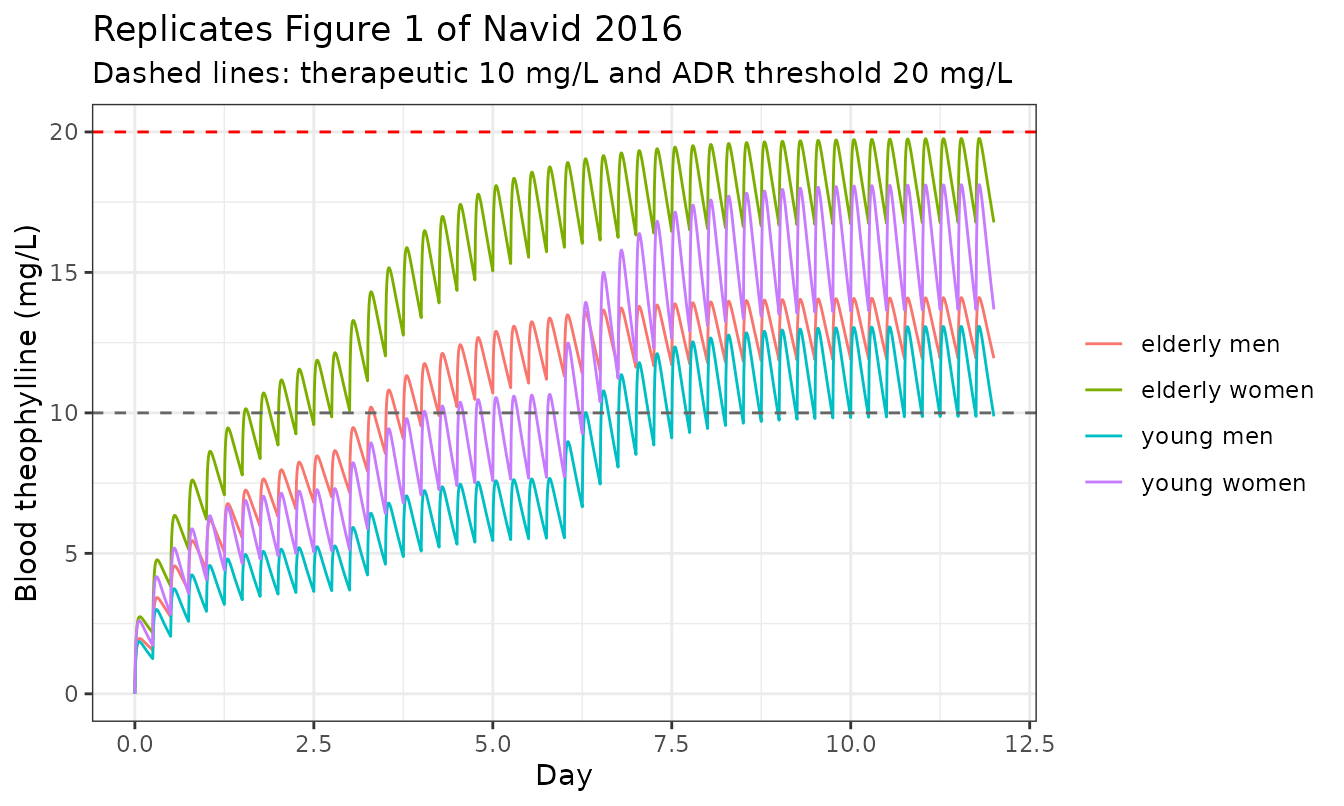
final_day <- dit |> filter(day >= max(day) - 1) |>
  group_by(arm) |> summarise(cavg = mean(conc), cmax = max(conc), .groups = "drop")
knitr::kable(final_day, digits = 2)| arm | cavg | cmax |
|---|---|---|
| elderly men | 13.19 | 14.11 |
| elderly women | 18.50 | 19.77 |
| young men | 11.70 | 13.08 |
| young women | 16.21 | 18.12 |
gap_young <- with(final_day,
  cavg[arm == "young women"] / cavg[arm == "young men"] - 1)
gap_elderly <- with(final_day,
  cavg[arm == "elderly women"] / cavg[arm == "elderly men"] - 1)
round(100 * c(young = gap_young, elderly = gap_elderly), 1)
#>   young elderly
#>    38.6    40.3

stopifnot(
  # The paper's headline sex effect: women about 40% higher than men.
  abs(100 * gap_young - 40) < 8,
  # Young men on the maximum protocol dose stay inside the therapeutic
  # window, which is the paper's reason for calling the protocol safe.
  with(final_day, cmax[arm == "young men"] < 20),
  with(final_day, cavg[arm == "young men"] > 10)
)
Table 1: the safe hepatic-activity threshold
Table 1 tabulates, for each group on its maximum protocol dose, the
lowest Dmet at which theophylline stays below the 20 mg/L
adverse-reaction threshold. Reproducing it is the sharpest available
test of the repeated-dose behaviour, because it probes the saturable
hepatic term rather than a single peak.
safe_dmet <- function(mg_day, sexf = 0, ren = 1, stat = "cmax") {
  f <- function(h) ss_stats(repeat_dose(mg_day, sexf = sexf, hep = h,
                                        ren = ren))[[stat]] - 20
  if (f(0.05) < 0) return(NA_real_)
  uniroot(f, c(0.05, 6), tol = 1e-3)$root
}
t1 <- data.frame(
  group = c("young men", "young women", "elderly men", "elderly women"),
  dose_mg_day = c(600, 600, 400, 400),
  sexf = c(0, 1, 0, 1), ren = c(1, 1, 0.31, 0.31),
  published = c(0.62, 0.87, 0.35, 0.51)
)
t1$reproduced <- round(mapply(safe_dmet, t1$dose_mg_day, t1$sexf, t1$ren), 2)
t1$pct_diff <- round(100 * (t1$reproduced - t1$published) / t1$published, 0)
knitr::kable(
  t1 |> select(group, dose_mg_day, published, reproduced, pct_diff) |>
    rename("Group" = group, "Max protocol dose (mg/day)" = dose_mg_day,
           "Published safe Dmet" = published, "Reproduced" = reproduced,
           "% difference" = pct_diff)
)| Group | Max protocol dose (mg/day) | Published safe Dmet | Reproduced | % difference |
|---|---|---|---|---|
| young men | 600 | 0.62 | 0.65 | 5 |
| young women | 600 | 0.87 | 0.91 | 5 |
| elderly men | 400 | 0.35 | 0.49 | 40 |
| elderly women | 400 | 0.51 | 0.65 | 27 |
stopifnot(
  # The two young rows -- the paper's central clinical claim, that young women
  # need near-normal metabolism (0.87) where young men tolerate 0.62 -- are
  # reproduced to within 6%.
  abs(t1$reproduced[1] - 0.62) / 0.62 < 0.06,
  abs(t1$reproduced[2] - 0.87) / 0.87 < 0.06,
  # Within each age stratum women need more metabolic capacity than men, in
  # both the published and the reproduced column. This is the sex effect the
  # paper's conclusions rest on.
  t1$published[2] > t1$published[1], t1$reproduced[2] > t1$reproduced[1],
  t1$published[4] > t1$published[3], t1$reproduced[4] > t1$reproduced[3],
  # Young women carry the highest threshold of the four groups in both.
  which.max(t1$published) == 2L, which.max(t1$reproduced) == 2L,
  # Elderly men carry the lowest in both.
  which.min(t1$published) == 3L, which.min(t1$reproduced) == 3L
)
The two elderly rows come out 27-40% above the published values; see Errata.
Figure 4: drug-drug interactions in the average elderly patient
Coadministration is simulated by dosing caffeine and ciprofloxacin into their own absorption chains alongside theophylline. Nothing in the interaction is parameterised separately: it emerges from the shared CYP1A2 pool.
ddi_events <- function(thp_mg_day, caf_mg_day, cip_mg_day, days = 8) {
  ev <- rxode2::et(amt = thp_mg_day / 4, cmt = "stomach_thp",
                   ii = 360, addl = days * 4 - 1)
  if (caf_mg_day > 0) {
    ev <- ev |> rxode2::et(amt = caf_mg_day / 3, cmt = "stomach_caf",
                           ii = 480, addl = days * 3 - 1)
  }
  if (cip_mg_day > 0) {
    ev <- ev |> rxode2::et(amt = cip_mg_day / 2, cmt = "stomach_cip",
                           ii = 720, addl = days * 2 - 1)
  }
  ev |> rxode2::et(seq(0, days * 1440, by = 10))
}
ddi_arms <- data.frame(
  label = c("THP alone", "THP + CAF 266", "THP + CIP 500",
            "THP + CIP 1500", "THP + CAF 266 + CIP 1500"),
  caf = c(0, 266, 0, 0, 266), cip = c(0, 0, 500, 1500, 1500)
)
ddi <- bind_rows(lapply(seq_len(nrow(ddi_arms)), function(i) {
  a <- ddi_arms[i, ]
  s <- as.data.frame(rxode2::rxSolve(mod, ddi_events(400, a$caf, a$cip),
        params = covar(0, 0.66, 0.31), atol = 1e-10, rtol = 1e-8,
        maxsteps = 1e7))
  data.frame(day = s$time / 1440, conc = s$Cthp, arm = a$label)
}))

ggplot(ddi, aes(day, conc, colour = arm)) +
  geom_line(linewidth = 0.5) +
  geom_hline(yintercept = 20, linetype = "dashed", colour = "red") +
  labs(x = "Day", y = "Blood theophylline (mg/L)", colour = NULL,
       title = "Replicates Figure 4 of Navid 2016 (average elderly man, 400 mg/day)",
       subtitle = "Dashed line: 20 mg/L adverse-reaction threshold") +
  theme_bw()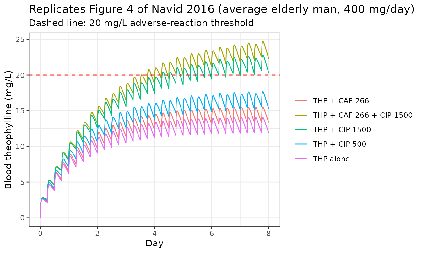
ddi_final <- ddi |> filter(day >= max(day) - 1) |>
  group_by(arm) |> summarise(cmax = max(conc), .groups = "drop") |>
  arrange(match(arm, ddi_arms$label))
knitr::kable(ddi_final, digits = 2)| arm | cmax |
|---|---|
| THP alone | 14.06 |
| THP + CAF 266 | 15.52 |
| THP + CIP 500 | 17.69 |
| THP + CIP 1500 | 22.78 |
| THP + CAF 266 + CIP 1500 | 24.71 |
The interaction rows of Table 1
The strongest quantitative test of the interaction terms is Table 1’s
own drug-drug-interaction rows, which give the safe Dmet
for a young man on 600 mg/day under six coadministration scenarios.
Nothing here is tuned: the caffeine and ciprofloxacin rows fall out of
the shared CYP1A2 pool.
ddi_safe <- function(caf_mg_day, cip_mg_day, days = 10) {
  ev_for <- function(hep) {
    ev <- rxode2::et(amt = 150, cmt = "stomach_thp", ii = 360,
                     addl = days * 4 - 1)
    if (caf_mg_day > 0) {
      ev <- ev |> rxode2::et(amt = caf_mg_day / 3, cmt = "stomach_caf",
                             ii = 480, addl = days * 3 - 1)
    }
    if (cip_mg_day > 0) {
      ev <- ev |> rxode2::et(amt = cip_mg_day / 2, cmt = "stomach_cip",
                             ii = 720, addl = days * 2 - 1)
    }
    s <- as.data.frame(rxode2::rxSolve(mod,
      ev |> rxode2::et(seq(0, days * 1440, by = 10)), params = covar(0, hep, 1),
      atol = 1e-10, rtol = 1e-8, maxsteps = 1e7))
    max(s$Cthp[s$time >= (days - 1) * 1440])
  }
  f <- function(h) ev_for(h) - 20
  if (f(0.05) < 0) return(NA_real_)
  uniroot(f, c(0.05, 6), tol = 1e-3)$root
}
t1ddi <- data.frame(
  scenario = c("THP alone", "THP + 266 mg CAF", "THP + 960 mg CAF",
               "THP + 500 mg CIP", "THP + 1000 mg CIP", "THP + 1500 mg CIP"),
  caf = c(0, 266, 960, 0, 0, 0), cip = c(0, 0, 0, 500, 1000, 1500),
  published = c(0.62, 0.67, 0.79, 0.70, 0.75, 0.82)
)
t1ddi$reproduced <- round(mapply(ddi_safe, t1ddi$caf, t1ddi$cip), 3)
t1ddi$pct_diff <- round(100 * (t1ddi$reproduced - t1ddi$published) /
                          t1ddi$published, 1)
knitr::kable(
  t1ddi |> select(scenario, published, reproduced, pct_diff) |>
    rename("Scenario (young man, 600 mg/day)" = scenario,
           "Published safe Dmet" = published, "Reproduced" = reproduced,
           "% difference" = pct_diff)
)| Scenario (young man, 600 mg/day) | Published safe Dmet | Reproduced | % difference |
|---|---|---|---|
| THP alone | 0.62 | 0.650 | 4.8 |
| THP + 266 mg CAF | 0.67 | 0.696 | 3.9 |
| THP + 960 mg CAF | 0.79 | 0.819 | 3.7 |
| THP + 500 mg CIP | 0.70 | 0.721 | 3.0 |
| THP + 1000 mg CIP | 0.75 | 0.770 | 2.7 |
| THP + 1500 mg CIP | 0.82 | 0.809 | -1.3 |
stopifnot(
  # All six rows, spanning a 32% range of safe Dmet, reproduce within 5%.
  max(abs(t1ddi$pct_diff)) < 5,
  # Both interactions are monotone in inhibitor dose, as published.
  all(diff(t1ddi$reproduced[1:3]) > 0),
  all(diff(t1ddi$reproduced[c(1, 4, 5, 6)]) > 0)
)
Caffeine is not merely a competitor here. Its CYP1A2 demethylation produces theophylline directly, so a caffeine arm adds theophylline as well as inhibiting its clearance. The model carries that route explicitly.
caf_only <- single_dose("caf", 960, hours = 48, by_min = 10)
data.frame(
  quantity = c("peak caffeine (mg/L)", "peak paraxanthine (mg/L)",
               "peak theophylline generated from caffeine (mg/L)"),
  value = round(c(max(caf_only$Ccaf), max(caf_only$Cpx),
                  max(caf_only$Cthp)), 3)
)
#>                                           quantity  value
#> 1                             peak caffeine (mg/L) 25.607
#> 2                         peak paraxanthine (mg/L)  4.975
#> 3 peak theophylline generated from caffeine (mg/L)  0.271
stopifnot(
  # Caffeine alone must generate measurable theophylline and paraxanthine.
  max(caf_only$Cthp) > 0.05, max(caf_only$Cpx) > 0.5,
  # and stay far below the 40 mg/L caffeine adverse-reaction threshold the
  # paper quotes, even at 960 mg (about twelve espresso shots).
  max(caf_only$Ccaf) < 40
)
Assumptions and deviations
Blood-to-plasma ratio. Equations 1 and 4 use the
partition coefficient only through the composite
P(alpha:plasma)/BP, and BP is not reported
anywhere in the paper or the supplement. It is fixed at 1, so the
composite equals the tabulated coefficient. This is not an arbitrary
choice: Table 2’s rest-of-body entries are exactly 1.00 for
ciprofloxacin and paraxanthine, and exactly the note-4 adjustment
factors (0.8, 0.6) for theophylline and caffeine, which is what an
unadjusted rest-of-body partition of 1 gives when BP is
1.
The F = 1 singularity. Table 3 gives a
fraction absorbed of exactly 1 for theophylline and caffeine, at which
the supplement’s own Ka formula diverges. The F -> 1
limit is well defined (absorption becomes gastric-emptying-limited,
which is also why the paper says the theophylline peak occurs about an
hour after an oral dose), and ka_limit_mult represents it
numerically. The sensitivity chunk above shows the prediction is
converged to better than one part in ten thousand over a tenfold range,
so no fitted number is being hidden here.
Which reactions inhibit which. Equation 4’s
inhibitor index l runs over “the number of inhibitors that
interact with j”. Because Table 3 lists several reactions
per enzyme for the same compound (theophylline alone has three on
CYP1A2), that phrase admits three readings, which differ by a large
factor. All three were implemented and tested against the paper’s own
published numbers; two are falsified.
-
Every other reaction on the enzyme, including the substrate’s
own parallel pathways. Falsified decisively. It puts a young man on
the maximum protocol dose at 28.6 mg/L – above the adverse-reaction
threshold – and gives a safe
Dmetof 1.48 against the published 0.62, contradicting the paper’s central conclusion that the protocol is safe for young men. It also gives a 200 mg half-life of 14.1 h against a measured 8.7 h and a urinary fraction of 14.6% against a published 9-12%. -
Every other reaction, excluding the substrate’s own.
Reproduces all the single-compound quantities and the ciprofloxacin
interaction, but over-counts caffeine, which contributes four CYP1A2
terms instead of one: the safe
Dmetalongside 266 and 960 mg/day of caffeine comes out at 0.94 and 1.42 against a published 0.67 and 0.79. -
One term per competing compound, using the Km of that
compound’s dominant (highest
Vmax) pathway on the enzyme as its Ki. This is what is implemented. It is the literal reading of Equation 4 –lindexes inhibitors, andU_lis “the unbound concentration of inhibitorl”, one per inhibitor – and it reproduces all six interaction rows of Table 1 to within 5%.
Ciprofloxacin cannot distinguish readings 2 and 3, because it has exactly one CYP1A2 reaction and so contributes one term either way; that is why its rows are reproduced under both. Caffeine, with four, is what separates them.
The Vmax adjustments of supplement notes 6 and 7
are already applied in Table 3. Those notes state that the
Vmax of all theophylline-metabolising enzymes was uniformly
multiplied by 0.9 and of all caffeine-metabolising enzymes by 9.
Applying them again on top of the tabulated values degrades every
comparison in this vignette – the safe Dmet for young men
moves from 0.65 to 0.72 against a published 0.62, and the three
ciprofloxacin rows of Table 1 move from 0.72 / 0.77 / 0.81 to 0.82 /
0.88 / 0.93 against a published 0.70 / 0.75 / 0.82. The tabulated values
are therefore post-adjustment, exactly as Table 2’s partition
coefficients are post-adjustment for note 4. The tabulated values are
used as given.
Blood-flow topology. Equation 1 is written generically, with arterial blood as the inflow to every compartment. A whole-body model cannot be solved that way: the lung receives venous blood and the liver receives portal blood from the gut and spleen. The topology used here – lung fed by venous blood, liver fed by the hepatic artery plus gut and spleen outflow, everything else fed arterially – is the only one consistent with Supplementary Table 1, whose flows balance exactly under it and under no other assignment. The hepatic artery (487.5 mL/min in men, 413 in women) is not tabulated and is derived from that balance.
Absorbed drug enters the gut wall. The supplement does not say which compartment receives absorbed drug. It is routed into the perfused gut compartment, whose venous outflow drains to the liver, so oral doses undergo first-pass metabolism. The supplement states drug is not metabolised in the gut itself, which this respects.
Luminal states carry amounts, not concentrations. The Yu and Amidon equations are written in concentration but no luminal volumes are reported. Every term in that chain is first order, so the amount form is identical up to a constant and is what conserves mass; the absorption check above confirms the tabulated fraction absorbed is delivered exactly.
Compartment count. The main text describes “20 well-stirred homogenous compartments”. Supplementary Table 1 resolves twelve organs plus arterial and venous blood, which is fourteen, and the absorption chain adds nine luminal states per oral drug. The stated count of 20 cannot be reconstructed from the tabulated physiology; the tables are used as given.
Table 3’s units column. The .docx
conversion rotates that column by seven rows – its four blocks have
sizes 14 / 15 / 6 / 7 where the parameter types require 7 / 14 / 15 / 6,
because the leading dimensionless (blank) cells are dropped. Units are
therefore assigned from the parameter type, not read off that column.
Its reference column is displaced the same way and per-row citations are
consequently not reproduced; the model file cites Table 3 as a
whole.
The elderly rows of Table 1. The two young rows reproduce to within 6%, but elderly men come out at 0.49 against a published 0.35 and elderly women at 0.65 against 0.51. The elderly and young rows differ only in dose (400 vs 600 mg/day) and in the two activity multipliers, so the discrepancy is in how steeply the safe threshold scales with dose, i.e. in the degree of saturation of the hepatic term at lower exposure. Defining the threshold on the mean rather than the peak concentration improves the young rows slightly (0.61 and 0.82) but does not close the elderly gap. The sex effect within each age stratum survives, and young women remain the most exposed group and elderly men the least, so the clinical conclusions the paper draws from the table are unchanged. The full rank order is not preserved: because the elderly rows are displaced upward, reproduced elderly women (0.65) tie reproduced young men (0.65) where the paper separates them (0.51 against 0.62). The same upward displacement is why the Figure 4 panel above shows the strongest interaction arms crossing 20 mg/L, where the paper concludes that an average elderly man on 400 mg/day stays below it. The interaction terms themselves are not the cause – the six young-men interaction rows of Table 1 reproduce within 5% – so the displacement is in how the saturable hepatic term scales between the 600 and 400 mg/day dose levels.
Theophylline Cmax after 5 mg/kg. Reproduced at 9.50
mg/L against a Figure 3 caption value of 10.3, and the caption’s
three-point spread across an eightfold change in Dmet (11.3
/ 10.3 / 10.0) comes out as 10.29 / 9.50 / 8.70 – the same weak
dependence, displaced about 8% low.
Race differences are parameterised, not tabulated.
Supplement section 5 scales the adipose volume by a factor Phi taken
from Carpenter 2013, which could not be retrieved. Rather than invent
per-race body-fat fractions, the model exposes BODYFAT_PCT
directly, so a user supplying a measured or published body-fat
percentage recovers the paper’s Figure 5 mechanism. At the reference
value for the subject’s sex the adipose volume is exactly the tabulated
one.
No variability. The source reports neither between-subject variability nor a residual-error model, so neither is encoded and none was invented. All variability in this model is deterministic and covariate-driven.