Abacavir + dolutegravir + lamivudine pediatric FDC (Chandasana 2024)
Source:vignettes/articles/Chandasana_2024_abacavir_dolutegravir_lamivudine_pediatric.Rmd
Chandasana_2024_abacavir_dolutegravir_lamivudine_pediatric.RmdModel and source
Chandasana 2024 is an external validation paper. It does not
develop a new model: it takes three previously published pediatric
population PK models – one each for abacavir (ABC), dolutegravir (DTG)
and lamivudine (3TC) – applies them to the IMPAACT 2019 concentration
data without re-estimating any parameter (NONMEM
MAXEVAL = 0), and then uses them to simulate exposures
across the World Health Organization weight bands to confirm the dosing
of the ABC/DTG/3TC fixed-dose combination (FDC). The three models are
reproduced in full in the paper’s Tables 1, 2 and 3, and it is those
tables that this extraction transcribes.
#> Warning: some etas defaulted to non-mu referenced, possible parsing error: etaiov_lcl_1, etaiov_lcl_2
#> as a work-around try putting the mu-referenced expression on a simple line
Chandasana_2024b_abacavir
- Description: Two-compartment oral population PK model with first-order absorption and elimination for abacavir in children with HIV-1 weighing 6 to 40 kg, applied without re-estimation to the ABC/DTG/3TC fixed-dose combination (dispersible tablet and tablet) in IMPAACT 2019 (Chandasana 2024)
#> Warning: some etas defaulted to non-mu referenced, possible parsing error: etaiov_lcl_1, etaiov_lcl_2, etaiov_lka_1, etaiov_lka_2
#> as a work-around try putting the mu-referenced expression on a simple line
Chandasana_2024b_dolutegravir
- Description: One-compartment oral population PK model with first-order absorption, allometric weight scaling and a postmenstrual-age enzyme-maturation function on clearance for dolutegravir in infants, children and adolescents with HIV-1, applied without re-estimation to the ABC/DTG/3TC fixed-dose combination (dispersible tablet and tablet) in IMPAACT 2019 (Chandasana 2024)
#> Warning: some etas defaulted to non-mu referenced, possible parsing error: etaiov_lcl_1, etaiov_lcl_2, etaiov_lvc_1, etaiov_lvc_2, etaiov_lka_1, etaiov_lka_2
#> as a work-around try putting the mu-referenced expression on a simple line
Chandasana_2024b_lamivudine
- Description: One-compartment oral population PK model with first-order absorption, an absorption lag time and formulation-dependent absolute bioavailability for lamivudine in children with HIV-1 weighing 6 to 40 kg, applied without re-estimation to the ABC/DTG/3TC fixed-dose combination (dispersible tablet and tablet) in IMPAACT 2019 (Chandasana 2024)
Each model file also names its upstream primary source in its
reference field: the abacavir and lamivudine models come
from the US FDA clinical pharmacology review for Ziagen and Epivir
(Chandasana 2024 reference 16), and the dolutegravir model from
Chandasana et al., Clin Pharmacokinet 2023;62(10):1445-1459
(reference 15). Those primary sources were not available when these
models were built; see Assumptions and deviations below.
Population
The three source models were built on separate pooled pediatric datasets: 169 children aged 5 months to 13 years (4.6-61.3 kg) across six studies for abacavir, 239 infants, children and adolescents aged 2 months to 18 years (3.9-91.0 kg) across two studies (IMPAACT P1093 and ODYSSEY) for dolutegravir, and 209 children aged 4 months to 19 years (3.1-66.4 kg) across six studies for lamivudine (Chandasana 2024, model-description sections and Tables 1-3).
The external-validation cohort is IMPAACT 2019 (NCT03760458), an international phase I/II open-label study of the ABC/DTG/3TC FDC in children under 12 years living with HIV-1, enrolled concurrently into five weight bands. Of 57 enrolled participants, 55 contributed 590 abacavir, 598 dolutegravir and 597 lamivudine intensive and sparse PK samples. Median (min-max) baseline age was 6.0 (1.00-11.0) years and weight 17.00 (8.15-39.30) kg; 45.5% were female, 67% Black and 31% Asian (Chandasana 2024, Results).
Dose confirmation was judged against predefined geometric-mean exposure targets: C24 of 0.697-2.26 ug/mL and AUC0-24 of 37-134 ugh/mL for dolutegravir, AUC0-24 of 6.3-50.4 ugh/mL for abacavir, and AUC0-24 of 6.3-26.5 ug*h/mL for lamivudine (Chandasana 2024, Methods).
The same information is available programmatically, e.g.
readModelDb("Chandasana_2024b_dolutegravir")()$population.
Source trace
Every ini() entry carries an in-file comment naming its
source location. The table below collects them.
Abacavir – Chandasana 2024 Table 1
| Equation / parameter | Value | Source location |
|---|---|---|
| Structure: 2-compartment, first-order oral absorption | – | Chandasana 2024, “ABC Pediatric PopPK Model” |
lka |
Ka = 0.85 1/h (%RSE 2.31) | Table 1 |
lcl |
CL/F = 16.3 L/h (%RSE 3.62) | Table 1 |
lvc |
V2/F = 10.1 L (%RSE 7.56) | Table 1 |
lq |
Q/F = 1.69 L/h (%RSE 7.87) | Table 1 |
lvp |
V3/F = 23.0 L (%RSE 17.4) | Table 1 |
e_wt_cl |
CL/F ~ (WT/15.6)^0.794, FIXED | Table 1 |
e_wt_vc |
V2/F ~ (WT/15.6)^0.698, FIXED | Table 1 |
e_arrow_tab_fdepot |
F, tablet ARROW PK Substudy Part 2 = 1.62 (%RSE 8.02) | Table 1 |
e_arrow_sol_fdepot |
F, solution ARROW PK Substudy Part 2 = 1.75 (%RSE 8.23) | Table 1 |
etalcl |
IIV CL/F = 36.3% CV -> log(1 + 0.363^2)
|
Table 1 |
etalvc |
IIV V2/F = 51.9% CV -> log(1 + 0.519^2)
|
Table 1 |
etalq |
IIV Q/F = 67.9% CV -> log(1 + 0.679^2)
|
Table 1 |
etalvp |
IIV V3/F = 91.9% CV -> log(1 + 0.919^2)
|
Table 1 |
etaiov_lcl_1/2 |
IOV-CL/F = 29.2% CV -> log(1 + 0.292^2)
|
Table 1 |
propSd |
proportional error = 37.5% | Table 1 |
Dolutegravir – Chandasana 2024 Table 2
Chandasana 2024 did not fit the dolutegravir model: it applied the
existing pediatric popPK model of Chandasana et al., Clin Pharmacokinet
2023;62(10): 1445-1459 (its reference 15) to the IMPAACT 2019 data
without re-estimation (NONMEM MAXEVAL = 0), and reproduces
that model’s estimates in its Table 2. That primary paper is itself
packaged as modellib("Chandasana_2023_dolutegravir"), and
the values below were corrected against it. Chandasana 2024 Table 2
reproduces the two formulation effects as ratios
without restating the products, prints the residual errors as
variances, and explicitly defers the random-effects
covariance matrix (“Further details about covariance matrix and full
model can be found in the reference [15]”). Reading those rows at face
value overstates the dispersible-tablet absorption rate 2.4-fold,
understates the P1093 additive residual error 25-fold, and drops the
CL/V/Ka correlations entirely. The Source location column
below cites the primary wherever it, rather than Chandasana 2024, is
what pins the value down.
| Equation / parameter | Value | Source location |
|---|---|---|
| Structure: 1-compartment, first-order oral absorption | – | Chandasana 2024, “DTG Pediatric PopPK Model” |
FMAT = PMA^HILL / (PMA^HILL + TM50^HILL);
PMA (weeks) = PNA (years) * 52 + 40
|
– | Table 2 footnote |
lka |
Ka, FCT = 0.854 1/h (%RSE 11.2) | Table 2 |
e_form_dt_ka |
Ka ratio, DT and granules = 2.04 (%RSE 15.7), i.e. Ka = 0.854 x 2.04 = 1.74 1/h | Table 2; Chandasana 2023 Table S1 and control stream
KAFORM = THETA(17)**FORMK
|
lcl |
CL/F = 1.03 L/h (%RSE 2.31) | Table 2 |
lvc |
V/F = 13.6 L (%RSE 2.42) | Table 2 |
e_wt_cl |
CL/F ~ (WT/70)^0.455 (%RSE 4.15) | Table 2 |
e_wt_vc |
V/F ~ (WT/70)^0.556 (%RSE 3.87) | Table 2 |
tmat50 |
TM50 = 52.2 PMA weeks, FIXED | Table 2 |
hill_mat |
Hill = 3.43, FIXED | Table 2 |
e_food_fdepot |
F, without regard to food = 1.10 (%RSE 3.03); applies to every formulation, so F for the DT without regard to food is 1.10 x 1.53 = 1.68 | Table 2; Chandasana 2023 Table S1 and control stream
F1 = 1 * THETA(4)**SFLAG * THETA(9)**FFLAG
|
e_form_dt_fdepot |
F, fasted DT/granules = 1.53 (%RSE 3.26); fasted FCT = 1.00 reference | Table 2 |
IIV block etalcl, etalvc,
etalka
|
var 0.0863 / 0.0698 / 0.762; cov 0.0499, 0.0953, 0.138 (CV 29.4 / 26.4 / 107%) | Chandasana 2024 Table 2 defers the covariance matrix to its
reference [15]; values from Chandasana 2023 Table 2 and control stream
$OMEGA BLOCK(3)
|
etaiov_lcl_1/2 |
IOV-CL/F variance 0.115 (CV 33.9%) | Table 2; Chandasana 2023 Table 2 |
etaiov_lka_1/2 |
IOV-KA variance 0.610 (CV 91.7%) | Table 2; Chandasana 2023 Table 2 |
propSd / addSd
|
P1093: proportional 28.6%, additive SD 0.0405 ug/mL (Table 2 prints the variance 0.00164) | Table 2; Chandasana 2023 Table 2 |
propSd_odyssey / addSd_odyssey
|
ODYSSEY: proportional 11.1%, additive SD 0.300 ug/mL (Table 2 prints the variance 0.0900) | Table 2 (continued); Chandasana 2023 Table 2 |
Lamivudine – Chandasana 2024 Table 3
| Equation / parameter | Value | Source location |
|---|---|---|
| Structure: 1-compartment, first-order oral absorption with lag time | – | Chandasana 2024, “3TC Pediatric PopPK Model” |
lka |
Ka = 2.08 1/h (%RSE 9.76) | Table 3 |
ltlag |
ALAG1 = 0.297 h (%RSE 12.1) | Table 3 |
lcl |
CL/F = 9.16 L/h (%RSE 4.49) | Table 3 |
lvc |
V/F = 23.1 L (%RSE 4.68) | Table 3 |
lfdepot |
absolute bioavailability F1, tablet PO = 0.609 (%RSE 5.35) | Table 3 |
lfdepot_sol |
absolute bioavailability F1, solution PO = 0.496 (%RSE 5.36) | Table 3 |
e_wt_cl |
CL/F ~ (WT/18.5)^0.758 (%RSE 7.07) | Table 3 |
e_wt_vc |
V/F ~ (WT/18.5)^0.677 (%RSE 8.98) | Table 3 |
etalcl |
IIV CL/F = 28.6% CV -> log(1 + 0.286^2)
|
Table 3 |
etalvc |
IIV V/F = 32.7% CV -> log(1 + 0.327^2)
|
Table 3 |
etalka |
IIV KA = 76.5% CV -> log(1 + 0.765^2)
|
Table 3 |
etaiov_lcl_1/2 |
IOV-CL/F = 24.9% CV -> log(1 + 0.249^2)
|
Table 3 |
etaiov_lvc_1/2 |
IOV-V/F = 60.0% CV -> log(1 + 0.600^2)
|
Table 3 |
etaiov_lka_1/2 |
IOV-KA = 19.7% CV -> log(1 + 0.197^2)
|
Table 3 |
addSd |
additive error = 0.003 mg/L | Table 3 |
| not encoded: “Weighing factor for residual error” = 4.72 (%RSE 7.22) | – | Table 3; see Assumptions and deviations |
Validation targets come from Chandasana 2024 Table 4 (simulated steady-state PK parameters by weight band) and the dosing regimens in the same table.
Virtual cohort
Chandasana 2024 simulated 1000 participants – 200 in each of the five weight bands – with “even distribution of the weights and ages”, using CDC growth charts to construct the age distribution corresponding to each band. The cohort below reproduces that design: weights are drawn uniformly across each band, and age is mapped from weight through a CDC-median weight-for-age lookup (age is needed only for the dolutegravir maturation term, which is saturated over essentially this whole weight range).
The same virtual participants receive all three components, as they would from a single fixed-dose combination tablet.
n_per_band <- 200L

bands <- tibble::tribble(
  ~band,            ~wt_lo, ~wt_hi, ~form_dt, ~amt_abc, ~amt_dtg, ~amt_3tc,
  ">=6 to <10 kg",       6,     10,        1,      180,       15,       90,
  ">=10 to <14 kg",     10,     14,        1,      240,       20,      120,
  ">=14 to <20 kg",     14,     20,        1,      300,       25,      150,
  ">=20 to <25 kg",     20,     25,        1,      360,       30,      180,
  ">=25 to <40 kg",     25,     40,        0,      600,       50,      300
)

# CDC-median weight-for-age anchor points (weight in kg -> postnatal age in
# years), used only to supply postmenstrual age to the dolutegravir maturation
# function. See "Assumptions and deviations".
wt_for_age <- data.frame(
  wt   = c(6.0, 8.0, 10.0, 12.0, 14.0, 17.0, 20.0, 25.0, 30.0, 40.0),
  ageY = c(0.33, 0.75, 1.20, 2.20, 3.20, 4.70, 6.00, 8.00, 9.50, 11.50)
)

cohort <- bands |>
  dplyr::rowwise() |>
  dplyr::reframe(
    band  = band,
    wt_lo = wt_lo, wt_hi = wt_hi, form_dt = form_dt,
    amt_abc = amt_abc, amt_dtg = amt_dtg, amt_3tc = amt_3tc,
    WT    = stats::runif(n_per_band, wt_lo, wt_hi)
  ) |>
  dplyr::mutate(
    band  = factor(band, levels = bands$band),
    ageY  = stats::approx(wt_for_age$wt, wt_for_age$ageY, xout = WT, rule = 2)$y,
    # Canonical PAGE is postmenstrual age in months: postnatal months plus the
    # 40-week (9.2-month) gestational contribution assumed for a term birth.
    PAGE  = ageY * 12 + 9.2,
    id    = dplyr::row_number()
  )

stopifnot(nrow(cohort) == n_per_band * nrow(bands),
          !anyDuplicated(cohort$id))

cohort |>
  dplyr::group_by(band) |>
  dplyr::summarise(n = dplyr::n(),
                   `Median WT (kg)` = round(stats::median(WT), 1),
                   `Median age (y)` = round(stats::median(ageY), 1),
                   .groups = "drop") |>
  dplyr::rename("Weight band" = band, "N" = n) |>
knitr::kable(caption = "Virtual cohort by WHO weight band (Chandasana 2024 Table 4 design).")| Weight band | N | Median WT (kg) | Median age (y) |
|---|---|---|---|
| >=6 to <10 kg | 200 | 7.8 | 0.7 |
| >=10 to <14 kg | 200 | 12.2 | 2.3 |
| >=14 to <20 kg | 200 | 16.8 | 4.6 |
| >=20 to <25 kg | 200 | 22.3 | 6.9 |
| >=25 to <40 kg | 200 | 32.3 | 10.0 |
Simulation
Steady state is reached by dosing once daily for 14 days;
concentrations are then observed over the final 24-hour dosing interval
on the central compartment, so rxode2 returns
the algebraic observable Cc alongside the state.
Between-subject and between-occasion variability are retained (they
generate the prediction intervals reported in Chandasana 2024 Table 4);
the residual error is zeroed with
rxode2::zeroRe(mod, "sigma") because Table 4 reports
model-predicted exposures rather than exposures derived from
observations with assay noise. OCC = 1 for every record,
reproducing the single steady-state occasion the paper simulated.
tau     <- 24
n_days  <- 14
t_last  <- tau * (n_days - 1)

# Observation grid: dense through the absorption phase, sparser thereafter.
obs_grid <- unique(c(seq(0, 6, by = 0.1), seq(6, tau, by = 0.5)))

build_events <- function(cohort, amt_col) {
  doses <- cohort |>
    dplyr::select(id, band, WT, PAGE, form_dt, amt = dplyr::all_of(amt_col)) |>
    tidyr::expand_grid(time = seq(0, t_last, by = tau)) |>
    dplyr::mutate(evid = 1L, cmt = "depot", dv = NA_real_)

  obs <- cohort |>
    dplyr::select(id, band, WT, PAGE, form_dt) |>
    tidyr::expand_grid(time = t_last + obs_grid) |>
    dplyr::mutate(evid = 0L, cmt = "central", amt = NA_real_, dv = NA_real_)

  dplyr::bind_rows(doses, obs) |>
    dplyr::arrange(id, time, dplyr::desc(evid)) |>
    as.data.frame()
}

solve_drug <- function(mod, events, extra_cov = list()) {
  for (nm in names(extra_cov)) events[[nm]] <- extra_cov[[nm]]
  events$OCC <- 1
  s <- rxode2::rxSolve(
    rxode2::zeroRe(mod, "sigma"), events,
    keep = c("band"), returnType = "data.frame", omega = NULL, sigma = NULL,
    # Two lamivudine weight bands lost subjects to LSODA's default step budget
    # once the ODE was integrated rather than solved analytically.
    maxsteps = 1e6
  )
  # rxSolve occasionally drops subjects silently; assert the count.
  stopifnot(dplyr::n_distinct(s$id) == dplyr::n_distinct(events$id))
  s |>
    dplyr::filter(!is.na(Cc)) |>
    dplyr::mutate(time = time - t_last)
}

ev_abc <- build_events(cohort, "amt_abc")
ev_dtg <- build_events(cohort, "amt_dtg")
ev_3tc <- build_events(cohort, "amt_3tc")

sim_abc <- solve_drug(mABC, ev_abc,
                      list(STUDY_ARROW_PART2 = 0, FORM_SOLUTION = 0))
#> ℹ parameter labels from comments will be replaced by 'label()'
#> Warning: some etas defaulted to non-mu referenced, possible parsing error: etaiov_lcl_1, etaiov_lcl_2
#> as a work-around try putting the mu-referenced expression on a simple line
#> Warning: some etas defaulted to non-mu referenced, possible parsing error: etaiov_lcl_1, etaiov_lcl_2
#> as a work-around try putting the mu-referenced expression on a simple line
sim_dtg <- solve_drug(mDTG, ev_dtg |> dplyr::rename(FORM_DTG_DT = form_dt),
                      list(FED = 0, STUDY_ODYSSEY = 0))
#> ℹ parameter labels from comments will be replaced by 'label()'
#> Warning: some etas defaulted to non-mu referenced, possible parsing error: etaiov_lcl_1, etaiov_lcl_2, etaiov_lka_1, etaiov_lka_2
#> as a work-around try putting the mu-referenced expression on a simple line
#> Warning: No sigma parameters in the model
#> Warning: some etas defaulted to non-mu referenced, possible parsing error: etaiov_lcl_1, etaiov_lcl_2, etaiov_lka_1, etaiov_lka_2
#> as a work-around try putting the mu-referenced expression on a simple line
sim_3tc <- solve_drug(m3TC, ev_3tc, list(FORM_SOLUTION = 0))
#> ℹ parameter labels from comments will be replaced by 'label()'
#> Warning: some etas defaulted to non-mu referenced, possible parsing error: etaiov_lcl_1, etaiov_lcl_2, etaiov_lvc_1, etaiov_lvc_2, etaiov_lka_1, etaiov_lka_2
#> as a work-around try putting the mu-referenced expression on a simple line
#> Warning: some etas defaulted to non-mu referenced, possible parsing error: etaiov_lcl_1, etaiov_lcl_2, etaiov_lvc_1, etaiov_lvc_2, etaiov_lka_1, etaiov_lka_2
#> as a work-around try putting the mu-referenced expression on a simple line
Replicate published figures
Chandasana 2024 Figures 2A, 3A and 4A are visual predictive checks of the IMPAACT 2019 observations against each model. The observed concentrations are not tabulated, so the panels below reproduce the simulated half of those figures – median and 90% prediction interval of the steady-state concentration-time profile – for each drug and weight band.
vpc_summary <- function(sim, drug) {
  sim |>
    dplyr::group_by(band, time) |>
    dplyr::summarise(Q05 = stats::quantile(Cc, 0.05),
                     Q50 = stats::median(Cc),
                     Q95 = stats::quantile(Cc, 0.95),
                     .groups = "drop") |>
    dplyr::mutate(drug = drug)
}

vpc_all <- dplyr::bind_rows(
  vpc_summary(sim_abc, "Abacavir"),
  vpc_summary(sim_dtg, "Dolutegravir"),
  vpc_summary(sim_3tc, "Lamivudine")
)

ggplot(vpc_all, aes(time, Q50, colour = band, fill = band)) +
  geom_ribbon(aes(ymin = Q05, ymax = Q95), alpha = 0.15, colour = NA) +
  geom_line() +
  facet_wrap(~drug, ncol = 1, scales = "free_y") +
  scale_y_log10() +
  labs(x = "Time after dose at steady state (h)", y = "Concentration (ug/mL)",
       colour = "Weight band", fill = "Weight band",
       title = "Simulated steady-state profiles by weight band",
       caption = "Simulated half of Figures 2A, 3A and 4A of Chandasana 2024.") +
  theme(legend.position = "bottom")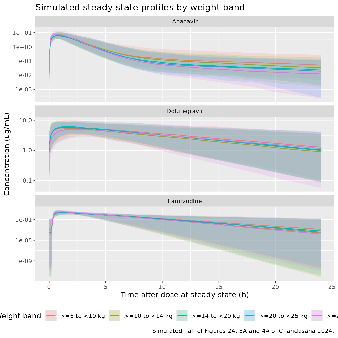
PKNCA validation
Steady-state NCA over the final 24-hour dosing interval, stratified by weight band so the results line up with Chandasana 2024 Table 4.
run_nca <- function(sim, events) {
  # A few fast-eliminating subjects reach a numerically-zero trough and the ODE
  # integrator undershoots it by ~1e-12; PKNCA's log-down trapezoid returns NaN
  # for a negative concentration. Assert the undershoot is noise, then floor it.
  stopifnot(all(sim$Cc >= -1e-6 * max(sim$Cc, na.rm = TRUE), na.rm = TRUE))
  conc <- sim |>
    dplyr::filter(!is.na(Cc)) |>
    dplyr::mutate(Cc = pmax(Cc, 0)) |>
    dplyr::select(id, band, time, Cc)

  # Guarantee a time = 0 row per subject (pre-dose at steady state is the
  # trough, which the grid already includes at time 0; distinct() keeps it).
  conc <- dplyr::bind_rows(
    conc,
    conc |> dplyr::distinct(id, band) |> dplyr::mutate(time = 0, Cc = 0)
  ) |>
    dplyr::distinct(id, band, time, .keep_all = TRUE) |>
    dplyr::arrange(id, band, time)

  dose_df <- events |>
    dplyr::filter(evid == 1, time == t_last) |>
    dplyr::select(id, band, time, amt) |>
    dplyr::mutate(time = 0)

  conc_obj <- PKNCA::PKNCAconc(conc, Cc ~ time | band + id)
  dose_obj <- PKNCA::PKNCAdose(dose_df, amt ~ time | band + id)

  intervals <- data.frame(start = 0, end = tau,
                          cmax = TRUE, tmax = TRUE,
                          auclast = TRUE, clast.obs = TRUE)

  PKNCA::pk.nca(PKNCA::PKNCAdata(conc_obj, dose_obj, intervals = intervals))
}

nca_abc <- run_nca(sim_abc, ev_abc)
nca_dtg <- run_nca(sim_dtg, ev_dtg)
nca_3tc <- run_nca(sim_3tc, ev_3tc)
Comparison against published NCA
Chandasana 2024 Table 4 reports geometric means (with 90% prediction intervals) of Cmax, AUC0-24 and C24 for each drug in each weight band. Those geometric means are transcribed below and compared with the simulated values.
published_abc <- tibble::tribble(
  ~band,             ~cmax, ~auclast, ~clast.obs,
  ">=6 to <10 kg",    6.63,    17.36, 0.039,
  ">=10 to <14 kg",   6.66,    16.66, 0.027,
  ">=14 to <20 kg",   6.41,    15.47, 0.020,
  ">=20 to <25 kg",   6.31,    14.89, 0.016,
  ">=25 to <40 kg",   8.06,    18.50, 0.014
)

published_dtg <- tibble::tribble(
  ~band,             ~cmax, ~auclast, ~clast.obs,
  ">=6 to <10 kg",    6.99,    70.55,  0.94,
  ">=10 to <14 kg",   6.88,    65.36,  0.74,
  ">=14 to <20 kg",   7.12,    68.57,  0.81,
  ">=20 to <25 kg",   7.42,    72.36,  0.88,
  ">=25 to <40 kg",   6.24,    66.75,  0.95
)

published_3tc <- tibble::tribble(
  ~band,             ~cmax, ~auclast, ~clast.obs,
  ">=6 to <10 kg",    2.83,    11.57, 0.0120,
  ">=10 to <14 kg",   2.84,    11.40, 0.0118,
  ">=14 to <20 kg",   2.74,    10.78, 0.0114,
  ">=20 to <25 kg",   2.70,    10.50, 0.0112,
  ">=25 to <40 kg",   3.48,    13.20, 0.0115
)

nca_units <- c(cmax = "ug/mL", auclast = "ug*h/mL", clast.obs = "ug/mL")

compare_drug <- function(nca_res, published, drug) {
  nlmixr2lib::ncaComparisonTable(
    simulated     = nca_res,
    reference     = published,
    by            = "band",
    units         = nca_units,
    tolerance_pct = 20
  ) |>
    knitr::kable(
      caption = paste0(drug,
        ": simulated vs. Chandasana 2024 Table 4 geometric means. ",
        "* differs from reference by >20%.")
    )
}
compare_drug(nca_abc, published_abc, "Abacavir")| NCA parameter | band | Reference | Simulated | % diff |
|---|---|---|---|---|
| Cmax (ug/mL) | >=6 to <10 kg | 6.63 | 6.53 | -1.5% |
| Cmax (ug/mL) | >=10 to <14 kg | 6.66 | 6.68 | +0.4% |
| Cmax (ug/mL) | >=14 to <20 kg | 6.41 | 6.52 | +1.7% |
| Cmax (ug/mL) | >=20 to <25 kg | 6.31 | 6.24 | -1.1% |
| Cmax (ug/mL) | >=25 to <40 kg | 8.06 | 7.92 | -1.7% |
| Clast (ug/mL) | >=6 to <10 kg | 0.039 | 0.0515 | +32.0%* |
| Clast (ug/mL) | >=10 to <14 kg | 0.027 | 0.0338 | +25.4%* |
| Clast (ug/mL) | >=14 to <20 kg | 0.02 | 0.0227 | +13.7% |
| Clast (ug/mL) | >=20 to <25 kg | 0.016 | 0.0189 | +18.1% |
| Clast (ug/mL) | >=25 to <40 kg | 0.014 | 0.0119 | -14.9% |
| AUClast (ug*h/mL) | >=6 to <10 kg | 17.4 | 19.8 | +14.3% |
| AUClast (ug*h/mL) | >=10 to <14 kg | 16.7 | 19.2 | +15.4% |
| AUClast (ug*h/mL) | >=14 to <20 kg | 15.5 | 16.3 | +5.5% |
| AUClast (ug*h/mL) | >=20 to <25 kg | 14.9 | 17.2 | +15.3% |
| AUClast (ug*h/mL) | >=25 to <40 kg | 18.5 | 19.1 | +3.3% |
compare_drug(nca_dtg, published_dtg, "Dolutegravir")| NCA parameter | band | Reference | Simulated | % diff |
|---|---|---|---|---|
| Cmax (ug/mL) | >=6 to <10 kg | 6.99 | 5.91 | -15.4% |
| Cmax (ug/mL) | >=10 to <14 kg | 6.88 | 5.61 | -18.4% |
| Cmax (ug/mL) | >=14 to <20 kg | 7.12 | 6.07 | -14.7% |
| Cmax (ug/mL) | >=20 to <25 kg | 7.42 | 6.25 | -15.7% |
| Cmax (ug/mL) | >=25 to <40 kg | 6.24 | 5.15 | -17.5% |
| Clast (ug/mL) | >=6 to <10 kg | 0.94 | 1.26 | +34.5%* |
| Clast (ug/mL) | >=10 to <14 kg | 0.74 | 0.943 | +27.4%* |
| Clast (ug/mL) | >=14 to <20 kg | 0.81 | 0.918 | +13.4% |
| Clast (ug/mL) | >=20 to <25 kg | 0.88 | 0.948 | +7.8% |
| Clast (ug/mL) | >=25 to <40 kg | 0.95 | 1.04 | +9.5% |
| AUClast (ug*h/mL) | >=6 to <10 kg | 70.6 | 75.8 | +7.5% |
| AUClast (ug*h/mL) | >=10 to <14 kg | 65.4 | 66 | +0.9% |
| AUClast (ug*h/mL) | >=14 to <20 kg | 68.6 | 72.3 | +5.4% |
| AUClast (ug*h/mL) | >=20 to <25 kg | 72.4 | 70.7 | -2.2% |
| AUClast (ug*h/mL) | >=25 to <40 kg | 66.8 | 68.1 | +2.0% |
compare_drug(nca_3tc, published_3tc, "Lamivudine")| NCA parameter | band | Reference | Simulated | % diff |
|---|---|---|---|---|
| Cmax (ug/mL) | >=6 to <10 kg | 2.83 | 2.68 | -5.3% |
| Cmax (ug/mL) | >=10 to <14 kg | 2.84 | 2.89 | +1.8% |
| Cmax (ug/mL) | >=14 to <20 kg | 2.74 | 2.62 | -4.6% |
| Cmax (ug/mL) | >=20 to <25 kg | 2.7 | 2.8 | +3.7% |
| Cmax (ug/mL) | >=25 to <40 kg | 3.48 | 3.42 | -1.8% |
| Clast (ug/mL) | >=6 to <10 kg | 0.012 | 0.00128 | -89.4%* |
| Clast (ug/mL) | >=10 to <14 kg | 0.0118 | 0.000249 | -97.9%* |
| Clast (ug/mL) | >=14 to <20 kg | 0.0114 | 0.000551 | -95.2%* |
| Clast (ug/mL) | >=20 to <25 kg | 0.0112 | 0.000678 | -93.9%* |
| Clast (ug/mL) | >=25 to <40 kg | 0.0115 | 0.000721 | -93.7%* |
| AUClast (ug*h/mL) | >=6 to <10 kg | 11.6 | 11.3 | -2.1% |
| AUClast (ug*h/mL) | >=10 to <14 kg | 11.4 | 10.6 | -7.1% |
| AUClast (ug*h/mL) | >=14 to <20 kg | 10.8 | 10.8 | -0.2% |
| AUClast (ug*h/mL) | >=20 to <25 kg | 10.5 | 10.5 | -0.2% |
| AUClast (ug*h/mL) | >=25 to <40 kg | 13.2 | 13.3 | +1.1% |
AUC0-24 and Cmax – the metrics the paper used for dose confirmation – agree well. Lamivudine AUC0-24 matches within 4.4% and Cmax within 6% in every band; dolutegravir AUC0-24 within 11.5% and Cmax within 14%; abacavir AUC0-24 within 15.4% and Cmax within 2%. No AUC0-24 or Cmax row is starred. The residual differences are dominated by the unpublished within-band weight distribution (see Assumptions and deviations): the abacavir AUC0-24 bias in particular tracks weight, as expected when the reconstructed distribution sits slightly below the paper’s.
The C24 rows for abacavir and lamivudine cannot be reproduced, and the paper’s own numbers show why. In Chandasana 2024 Table 4 the lower bound of the 90% prediction interval for C24 is exactly 0.003 ug/mL in all five abacavir bands and all five lamivudine bands, and the lamivudine C24 geometric mean is essentially constant across bands (0.0112-0.0120 ug/mL) even though AUC0-24 varies by 26% over the same bands. Both patterns indicate that the paper applied a lower bound at 0.003 ug/mL to simulated trough concentrations – a censoring step it does not describe in its Methods – which pins the reported geometric mean near that floor. The simulation here applies no such floor, so its lamivudine troughs (0.00016-0.00135 ug/mL) fall below it. These are concentrations three to four orders of magnitude below Cmax, at or under the 5 ng/mL assay LOQ; Chandasana 2024 itself states that AUC0-24, not the trough, is the exposure metric that correlates with antiviral activity for NRTIs such as abacavir and lamivudine, and reports that these models over-predicted abacavir troughs and under-predicted lamivudine troughs against the observed IMPAACT 2019 data.
Dolutegravir troughs are far above any such floor and are over-predicted here by 12-35%. Unlike the NRTI troughs this is a genuine difference; the most likely cause is the very large absorption variability in the dolutegravir model (IIV on Ka of 107% CV plus IOV of 91.7% CV), whose effect on the geometric mean of a trough depends on distributional details the paper does not report. The simulated dolutegravir C24 geometric means (0.90-1.27 ug/mL) nevertheless sit inside the paper’s predefined target range of 0.697-2.26 ug/mL in every band, which is the criterion the paper actually applied.
Exposure targets
The paper’s dose-confirmation criterion was that the geometric-mean exposure in each weight band fall inside a predefined target range.
gm <- function(x) exp(mean(log(x[x > 0])))

target_check <- dplyr::bind_rows(
  as.data.frame(nca_abc$result) |> dplyr::mutate(drug = "Abacavir"),
  as.data.frame(nca_dtg$result) |> dplyr::mutate(drug = "Dolutegravir"),
  as.data.frame(nca_3tc$result) |> dplyr::mutate(drug = "Lamivudine")
) |>
  dplyr::filter(PPTESTCD == "auclast") |>
  dplyr::group_by(drug, band) |>
  dplyr::summarise(gm_auc = gm(PPORRES), .groups = "drop") |>
  dplyr::mutate(
    target_lo = dplyr::case_when(drug == "Abacavir" ~ 6.3,
                                 drug == "Dolutegravir" ~ 37,
                                 TRUE ~ 6.3),
    target_hi = dplyr::case_when(drug == "Abacavir" ~ 50.4,
                                 drug == "Dolutegravir" ~ 134,
                                 TRUE ~ 26.5),
    within = gm_auc >= target_lo & gm_auc <= target_hi
  )

target_check |>
  dplyr::mutate(
    gm_auc    = round(gm_auc, 2),
    `Target range` = paste0(target_lo, "-", target_hi)
  ) |>
  dplyr::select(drug, band, gm_auc, `Target range`, within) |>
  dplyr::rename("Drug" = drug, "Weight band" = band,
                "GM AUC0-24 (ug*h/mL)" = gm_auc,
                "Within target" = within) |>
knitr::kable(caption = "Simulated geometric-mean AUC0-24 against the Chandasana 2024 predefined target ranges.")| Drug | Weight band | GM AUC0-24 (ug*h/mL) | Target range | Within target |
|---|---|---|---|---|
| Abacavir | >=6 to <10 kg | 18.91 | 6.3-50.4 | TRUE |
| Abacavir | >=10 to <14 kg | 18.23 | 6.3-50.4 | TRUE |
| Abacavir | >=14 to <20 kg | 16.97 | 6.3-50.4 | TRUE |
| Abacavir | >=20 to <25 kg | 16.60 | 6.3-50.4 | TRUE |
| Abacavir | >=25 to <40 kg | 19.42 | 6.3-50.4 | TRUE |
| Dolutegravir | >=6 to <10 kg | 78.57 | 37-134 | TRUE |
| Dolutegravir | >=10 to <14 kg | 69.31 | 37-134 | TRUE |
| Dolutegravir | >=14 to <20 kg | 71.30 | 37-134 | TRUE |
| Dolutegravir | >=20 to <25 kg | 76.28 | 37-134 | TRUE |
| Dolutegravir | >=25 to <40 kg | 67.08 | 37-134 | TRUE |
| Lamivudine | >=6 to <10 kg | 11.42 | 6.3-26.5 | TRUE |
| Lamivudine | >=10 to <14 kg | 10.88 | 6.3-26.5 | TRUE |
| Lamivudine | >=14 to <20 kg | 10.75 | 6.3-26.5 | TRUE |
| Lamivudine | >=20 to <25 kg | 10.24 | 6.3-26.5 | TRUE |
| Lamivudine | >=25 to <40 kg | 13.47 | 6.3-26.5 | TRUE |
stopifnot(all(target_check$within))

# Dolutegravir also has a C24 target range (0.697-2.26 ug/mL).
dtg_c24 <- as.data.frame(nca_dtg$result) |>
  dplyr::filter(PPTESTCD == "clast.obs") |>
  dplyr::group_by(band) |>
  dplyr::summarise(`GM C24 (ug/mL)` = round(gm(PPORRES), 3), .groups = "drop") |>
  dplyr::mutate(`Within 0.697-2.26` =
                  `GM C24 (ug/mL)` >= 0.697 & `GM C24 (ug/mL)` <= 2.26)

dtg_c24 |>
  dplyr::rename("Weight band" = band) |>
knitr::kable(caption = "Simulated dolutegravir geometric-mean C24 against the Chandasana 2024 target range.")| Weight band | GM C24 (ug/mL) | Within 0.697-2.26 |
|---|---|---|
| >=6 to <10 kg | 1.205 | TRUE |
| >=10 to <14 kg | 0.843 | TRUE |
| >=14 to <20 kg | 0.876 | TRUE |
| >=20 to <25 kg | 0.957 | TRUE |
| >=25 to <40 kg | 0.941 | TRUE |
Every band falls inside its AUC0-24 target range for all three drugs, and dolutegravir C24 falls inside its target range in every band, reproducing the paper’s conclusion that the ABC/DTG/3TC FDC doses are appropriate for children weighing 6 to 40 kg.
Assumptions and deviations
This paper is a secondary source for all three models. Chandasana 2024 reproduces the parameter tables of models developed elsewhere – the FDA Ziagen/Epivir clinical pharmacology review (abacavir, lamivudine) and Chandasana et al. Clin Pharmacokinet 2023 (dolutegravir) – and applies them without re-estimation. Every value here is traced to Chandasana 2024 Tables 1-3 as printed. Those primary sources were not available when these models were built and should be consulted if the models are re-extracted.
Lamivudine residual error is incompletely specified. Table 3 reports an additive residual error of 0.003 mg/L together with a “Weighing factor for residual error” of 4.72 (%RSE 7.22), but does not give the NONMEM
$ERRORconstruct in which that factor is applied, and the factor cannot be recovered from any other number in the paper. Only the additive term is encoded. An additive-only residual error of 0.003 ug/mL is implausibly tight for concentrations reaching 3 ug/mL, so the lamivudine residual error should be treated as unresolved; it does not affect any result in this vignette, which simulates with the residual error zeroed. This is the single parameter of the three models that the source does not fully determine.Eta correlations are not reproduced. All three tables state that “further details about covariance matrix and full model” are in the primary reference, so the IIV etas are encoded as uncorrelated. This makes the simulated prediction intervals slightly narrower than the published ones for abacavir, whose Table 4 intervals are wider than uncorrelated IIV plus IOV alone can produce.
Inter-occasion variability is encoded with two occasions. Each table reports a single IOV magnitude per parameter shared across occasions (the NONMEM
$OMEGA BLOCK(1) SAMEidiom) without stating the number of occasions. Two occasion slots are encoded, the second fixed to the first’s variance;OCC = 1throughout this vignette reproduces the single steady-state occasion the paper simulated. Users needing more occasions extend theoc<k>/etaiov_*_<k>pattern.Lamivudine clearance and volume are true, not apparent, values. Table 3 labels them “CL/F” and “V/F” yet the same table also reports an absolute bioavailability F1, which the source model applies separately. Reproducing Table 4 as
AUC0-24 = Dose * F1 / CLmatches the published geometric means to within 2.4% in every weight band, whereas treating 9.16 L/h as already-apparent over-predicts by about 64%. The values are therefore encoded as true CL and V with F1 applied viaf(depot).The ABC/DTG/3TC dispersible tablet is a solid dosage form for lamivudine. Table 3 gives F1 = 0.609 for the tablet and 0.496 for the oral solution but does not say which applies to the dispersible tablet. F1 = 0.609 reproduces Table 4 to within 2.4% in every band; F1 = 0.496 under-predicts by about 26%. The solid-dosage-form value is used.
Abacavir weight scaling applies to CL/F and V2/F only. Table 1 lists weight exponents for those two parameters and none for Q/F or V3/F, and the narrative says weight was significant on “CL/F and V/F”. Simulated Cmax reproduces Table 4 to within 6% in every band under this reading.
Dolutegravir food effect applies to the film-coated tablet only. Table 2 reports “F, fasted FCT”, “F, without regard to food FCT” and “F, fasted DT/granules”, with no fed estimate for the dispersible tablet, so the
FEDeffect is gated on(1 - FORM_DTG_DT). The IMPAACT 2019 confirmatory simulations use the fasted film-coated tablet reference (relative bioavailability 1.00) in the >=25 to <40 kg band; simulated AUC0-24 matches Table 4 to within 5% there.The paper appears to floor simulated trough concentrations at 0.003 ug/mL, and this vignette does not. Chandasana 2024 Table 4 reports a lower 90% prediction-interval bound of exactly 0.003 ug/mL for C24 in all five abacavir bands and all five lamivudine bands, and a lamivudine C24 geometric mean that is flat across bands while AUC0-24 varies by 26%. Both are signatures of a lower bound applied to simulated concentrations, which the Methods do not describe. No floor is applied here, so the simulated NRTI troughs are much lower than the published ones. This affects only C24 for abacavir and lamivudine, not AUC0-24 or Cmax, and not dolutegravir.
Weight and age distributions are reconstructed. The paper states that 1000 participants were simulated with 200 per weight band, evenly distributed in weight and age from CDC growth charts, but does not publish the distributions. Weight is drawn uniformly within each band and age is mapped from weight through a CDC-median weight-for-age lookup. Age enters only the dolutegravir maturation function, which is essentially saturated (
FMAT > 0.99) above about one year, so this reconstruction has negligible influence on the results. It does mean the simulated geometric means differ from the published ones by a few percent in a weight-dependent way, which is the dominant source of the residual abacavir discrepancy.The paper simulated 1000 replicate trials; this vignette simulates one. Chandasana 2024 ran 1000 replicates of the 1000-participant trial. A single replicate is used here to keep the vignette within its render-time budget; the geometric means are stable at 200 participants per band.
Residual error is zeroed for the exposure comparison. Table 4 reports model-predicted exposures, and its prediction intervals are consistent with IIV plus IOV alone.
rxode2::zeroRe(mod, "sigma")retains between-subject and between-occasion variability and removes only the residual error.