Miltefosine (Dorlo 2017)
Source:vignettes/articles/Dorlo_2017_miltefosine.Rmd
Dorlo_2017_miltefosine.RmdModel and source
- Citation: Dorlo TPC, Kip AE, Younis BM, Ellis SJ, Alves F, Beijnen JH, Njenga S, Kirigi G, Hailu A, Olobo J, Musa AM, Balasegaram M, Wasunna M, Karlsson MO, Khalil EAG. Visceral leishmaniasis relapse hazard is linked to reduced miltefosine exposure in patients from Eastern Africa: a population pharmacokinetic/pharmacodynamic study. J Antimicrob Chemother. 2017;72(11):3131-3140. doi:10.1093/jac/dkx283. ClinicalTrials.gov NCT01067443.
- Description: Two-compartment population PK model with first-order oral absorption for miltefosine in 95 Eastern African adults and children (>=7 years) with visceral leishmaniasis (Dorlo 2017), enrolled across three treatment centres in Kenya and Sudan and randomised to either a 28-day monotherapy regimen of oral miltefosine 2.5 mg/kg/day or a 10-day oral miltefosine 2.5 mg/kg/day arm combined with a single 10 mg/kg liposomal amphotericin B IV dose on day 1. CL/F, Q/F, Vc/F, and Vp/F are allometrically scaled on fat-free mass (exponents 0.75 and 1.0; reference FFM 53 kg). Relative bioavailability is structurally fixed at 100% from the end of the initial reduced absorption window onwards, and reduced by a typical 74.3% during the window itself (0 < t <= 7 days for monotherapy, 0 < t <= 1 day for the combination arm); the duration is regimen-dependent via the MIL_REGIMEN indicator. The combined-error residual model is proportional (31.0%) with additive component fixed at 0.001 ug/mL.
- Article: https://doi.org/10.1093/jac/dkx283
Population
The Dorlo 2017 model is a single-study population-PK analysis of oral
miltefosine in 95 Eastern African adults and children (>=7 years)
with parasitologically confirmed visceral leishmaniasis (kala-azar),
enrolled in NCT01067443 across three treatment centres in Kenya
(Kimalel) and Sudan (Dooka, Kassab). Patients were randomised to either
a 28-day miltefosine monotherapy regimen (oral miltefosine 2.5
mg/kg/day, maximum 150 mg/day; n=48) or a 10-day combination regimen of
the same miltefosine schedule preceded by a single IV dose of liposomal
amphotericin B (AmBisome, 10 mg/kg) on day 1 (n=47). The pooled cohort
had a median (range) age of 13 (7-41) years, body weight 32 (15-65) kg,
fat-free mass 29.9 (15.2-55.9) kg, with 13.7% female and 51%
malnourished by BMI / BMI-for-age z-score criteria. Forty-one of 95
(43.2%) patients were paediatric (>=7 and <12 years). See Dorlo
2017 Table 1 for the per-arm breakdown. The same information is
available programmatically via
rxode2::rxode(readModelDb("Dorlo_2017_miltefosine"))$population.
Source trace
The per-parameter origin is recorded as a trailing in-file comment
next to each ini() entry in
inst/modeldb/specificDrugs/Dorlo_2017_miltefosine.R. The
table below collects them in one place.
| Equation / parameter | Value | Source location (Dorlo 2017) |
|---|---|---|
lka (ka) |
1.49 1/day | Table 2 Pharmacokinetics ‘Absorption rate, k_a (/day)’ = 1.49 (RSE 17.7%) |
lcl (CL/F at FFM 53 kg) |
4.29 L/day | Table 2 ‘Clearance, CL/F (L/day)’ = 4.29 (RSE 3.22%) |
lvc (Vc/F at FFM 53 kg) |
51.7 L | Table 2 ‘Central volume of distribution, V_c/F (L)’ = 51.7 (RSE 4.33%) |
lq (Q/F at FFM 53 kg) |
0.0266 L/day | Table 2 ‘Intercompartmental clearance, Q/F (L/day)’ = 0.0266 (RSE 40.7%) |
lvp (Vp/F at FFM 53 kg) |
2.25 L | Table 2 ‘Peripheral volume of distribution, V_p/F (L)’ = 2.25 (RSE 14.1%) |
lfdepot |
log(1) FIXED | Table 2 ‘F (%, at end of treatment): 100 fixed’ |
lfred_mult |
log(0.257) | Table 2 ‘Reduction in F at baseline’ = -74.3% (RSE 4.68%) -> multiplier 1 - 0.743 = 0.257 |
e_ffm_cl_q |
0.75 FIXED | Table 2 footnote b: ‘allometrically scaled (power exponents of 0.75 and 1, respectively) based on fat-free mass’ |
e_ffm_vc_vp |
1.0 FIXED | Table 2 footnote b: same |
tlowf predicate |
7 days mono / 1 day combo | Table 2 footnote d: duration of reduction in F was ‘>0 to <=7 days for the monotherapy regimen and from >0 to <=1 day for the combination therapy regimen’ |
| Two-compartment ODE structure | n/a | Results ‘Pharmacokinetics of miltefosine’ paragraph 1; base structural model from Dorlo 2008 [ref 11] |
etalka |
log(1 + 0.680^2) = 0.379 | Table 2 BSV ‘Absorption rate, k_a’ = 68.0% CV (RSE 24.5%) |
etalcl |
log(1 + 0.170^2) = 0.0286 | Table 2 BSV ‘Clearance, CL/F’ = 17.0% CV (RSE 23.3%) |
etalfred_mult |
log(1 + 0.964^2) = 0.657 | Table 2 BSV ‘Reduction in F at baseline’ = 96.4% CV (RSE 19.5%) |
propSd |
0.310 | Table 2 ‘Residual proportional error (%)’ = 31.0 (RSE 5.74%) |
addSd |
0.001 ug/mL FIXED | Table 2 ‘Residual additive error (ug/mL)’ = 0.001 fixed |
Virtual cohort
Original observed concentrations are not publicly available. We simulate two cohorts that mirror the published trial arms: 60 patients on miltefosine monotherapy (28-day regimen) and 60 patients on the combination regimen (10-day regimen). Within each arm 30 are paediatric (7-11 years, median 9; body weight 16-30 kg, median 22) and 30 are adult (12-41 years, median 25; body weight 30-65 kg, median 45). Fat-free mass is derived from body weight, height, and sex by the Janmahasatian (2005) formula. All subjects receive 2.5 mg/kg/day rounded to the nearest 50 mg capsule, capped at 150 mg/day.
set.seed(2017)

janmahasatian_ffm <- function(wt_kg, ht_cm, sexf) {
  bmi <- wt_kg / (ht_cm / 100)^2
  # Janmahasatian 2005 (Clin Pharmacokinet 44:1051-1065):
  # male:   FFM = 9.27e3 * WT / (6.68e3 + 216 * BMI)
  # female: FFM = 9.27e3 * WT / (8.78e3 + 244 * BMI)
  male_ffm   <- 9.27e3 * wt_kg / (6.68e3 + 216 * bmi)
  female_ffm <- 9.27e3 * wt_kg / (8.78e3 + 244 * bmi)
  ifelse(sexf == 1L, female_ffm, male_ffm)
}

n_per_age <- 30L

make_cohort <- function(regimen_label, mil_regimen, id_offset) {
  paeds <- tibble(
    id          = id_offset + seq_len(n_per_age),
    age_yr      = round(runif(n_per_age, 7, 11)),
    wt_kg       = round(runif(n_per_age, 16, 30), 1),
    ht_cm       = round(runif(n_per_age, 115, 150)),
    sexf        = rbinom(n_per_age, 1, 0.137),
    age_group   = "paediatric"
  )
  adults <- tibble(
    id          = id_offset + n_per_age + seq_len(n_per_age),
    age_yr      = round(runif(n_per_age, 12, 41)),
    wt_kg       = round(runif(n_per_age, 30, 65), 1),
    ht_cm       = round(runif(n_per_age, 150, 180)),
    sexf        = rbinom(n_per_age, 1, 0.137),
    age_group   = "adult"
  )
  bind_rows(paeds, adults) %>%
    mutate(
      regimen     = regimen_label,
      MIL_REGIMEN = mil_regimen,
      FFM         = janmahasatian_ffm(wt_kg, ht_cm, sexf),
      daily_dose  = pmin(150, round(2.5 * wt_kg / 50) * 50),
      n_doses     = ifelse(mil_regimen == 1L, 28L, 10L)
    )
}

cohort <- bind_rows(
  make_cohort("Monotherapy 28-day", mil_regimen = 1L, id_offset = 0L),
  make_cohort("Combination 10-day", mil_regimen = 0L, id_offset = 2L * n_per_age)
) %>%
  mutate(regimen = factor(regimen,
                          levels = c("Monotherapy 28-day", "Combination 10-day")))
Build event table
Doses are daily; observations are placed on a dense grid spanning the treatment period plus the 60-day and 210-day landmark follow-up samples described in the paper’s blood-sample schedule.
sim_horizon <- 210

events <- cohort %>%
  rowwise() %>%
  do({
    row <- .
    dose_times <- seq(0, row$n_doses - 1, by = 1)
    doses <- tibble(
      id          = row$id,
      regimen     = row$regimen,
      age_group   = row$age_group,
      time        = dose_times,
      amt         = row$daily_dose,
      evid        = 1L,
      cmt         = "depot",
      FFM         = row$FFM,
      MIL_REGIMEN = row$MIL_REGIMEN
    )
    obs <- tibble(
      id          = row$id,
      regimen     = row$regimen,
      age_group   = row$age_group,
      time        = sort(unique(c(seq(0, 30, by = 0.25),
                                  seq(30, 60, by = 1),
                                  seq(60, sim_horizon, by = 5)))),
      amt         = 0,
      evid        = 0L,
      cmt         = "central",
      FFM         = row$FFM,
      MIL_REGIMEN = row$MIL_REGIMEN
    )
    bind_rows(doses, obs)
  }) %>%
  ungroup() %>%
  arrange(id, time, desc(evid))

stopifnot(!anyDuplicated(unique(events[, c("id", "time", "evid")])))
Simulate (typical value, no IIV)
We use a typical-value simulation (between-subject variability zeroed out) so the within-cohort spread reflects only weight / FFM and daily- dose-rounding differences, matching the way Dorlo 2017 presents the Figure 2 visual predictive checks for the population median trajectory.
mod     <- readModelDb("Dorlo_2017_miltefosine")
mod_typ <- rxode2::zeroRe(mod)

sim <- rxode2::rxSolve(
  mod_typ,
  events = events,
  keep   = c("regimen", "age_group", "FFM")
) %>%
  as.data.frame()
#> ℹ omega/sigma items treated as zero: 'etalka', 'etalcl', 'etalfred_mult'
#> Warning: multi-subject simulation without without 'omega'
Replicate Figure 2: concentration-time profiles by regimen
Figure 2 of Dorlo 2017 plots the 50th percentile (and 10th / 90th) of observed miltefosine concentrations vs time, by treatment arm, with insets showing the first 28 days. Below we plot the simulated typical trajectory by regimen.
sim %>%
  group_by(regimen, time) %>%
  summarise(
    Q10 = quantile(Cc, 0.10, na.rm = TRUE),
    Q50 = quantile(Cc, 0.50, na.rm = TRUE),
    Q90 = quantile(Cc, 0.90, na.rm = TRUE),
    .groups = "drop"
  ) %>%
  ggplot(aes(time, Q50)) +
  geom_ribbon(aes(ymin = Q10, ymax = Q90), alpha = 0.20, fill = "#4477aa") +
  geom_line(colour = "#4477aa") +
  geom_hline(yintercept = 10.6, linetype = "dashed", colour = "red") +
  geom_hline(yintercept =  2.01, linetype = "dotted", colour = "red") +
  facet_wrap(~regimen, scales = "free_y") +
  scale_y_log10() +
  labs(
    x       = "Time (days)",
    y       = "Miltefosine plasma concentration (ug/mL, log scale)",
    title   = "Simulated miltefosine concentration-time profile",
    subtitle = "2.5 mg/kg/day rounded to 50 mg capsules, capped at 150 mg/day",
    caption = paste(
      "Replicates Dorlo 2017 Figure 2 typical trajectory.",
      "Solid line = median, ribbon = 10th-90th percentile across the simulated cohort.",
      "Red dashed line = in-vitro EC90 (10.6 ug/mL); dotted = EC50 (2.01 ug/mL)."
    )
  )
#> Warning in scale_y_log10(): log-10 transformation introduced infinite values.
#> log-10 transformation introduced infinite values.
#> log-10 transformation introduced infinite values.
#> log-10 transformation introduced infinite values.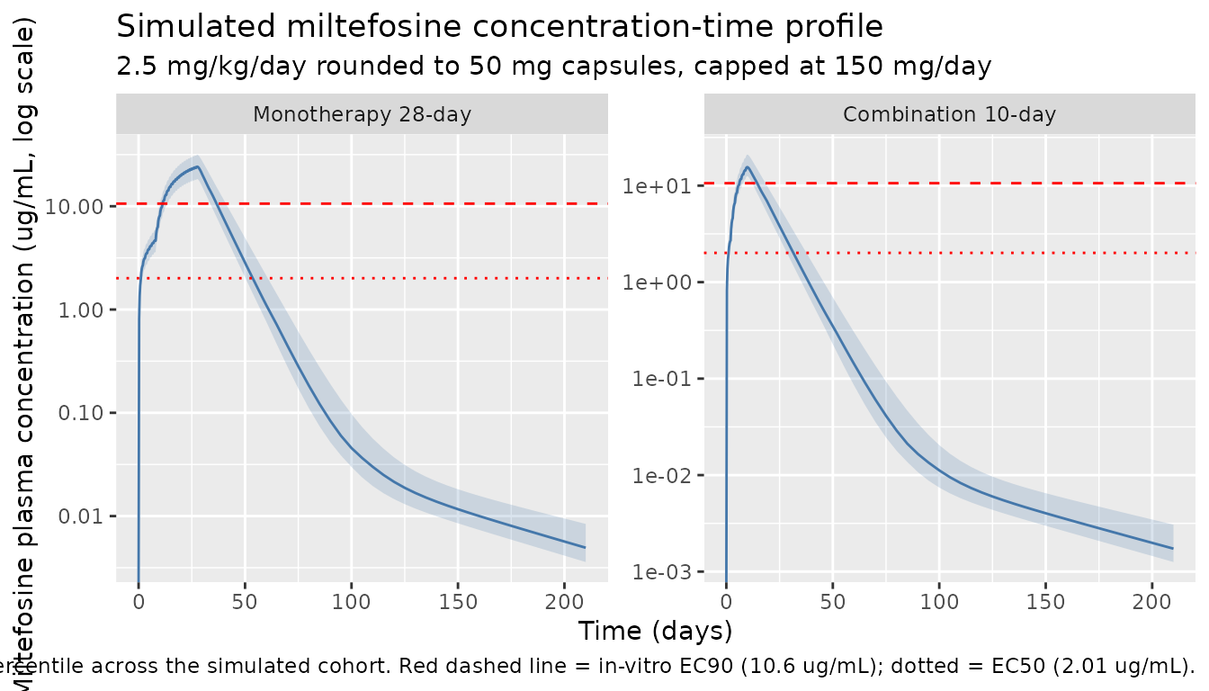
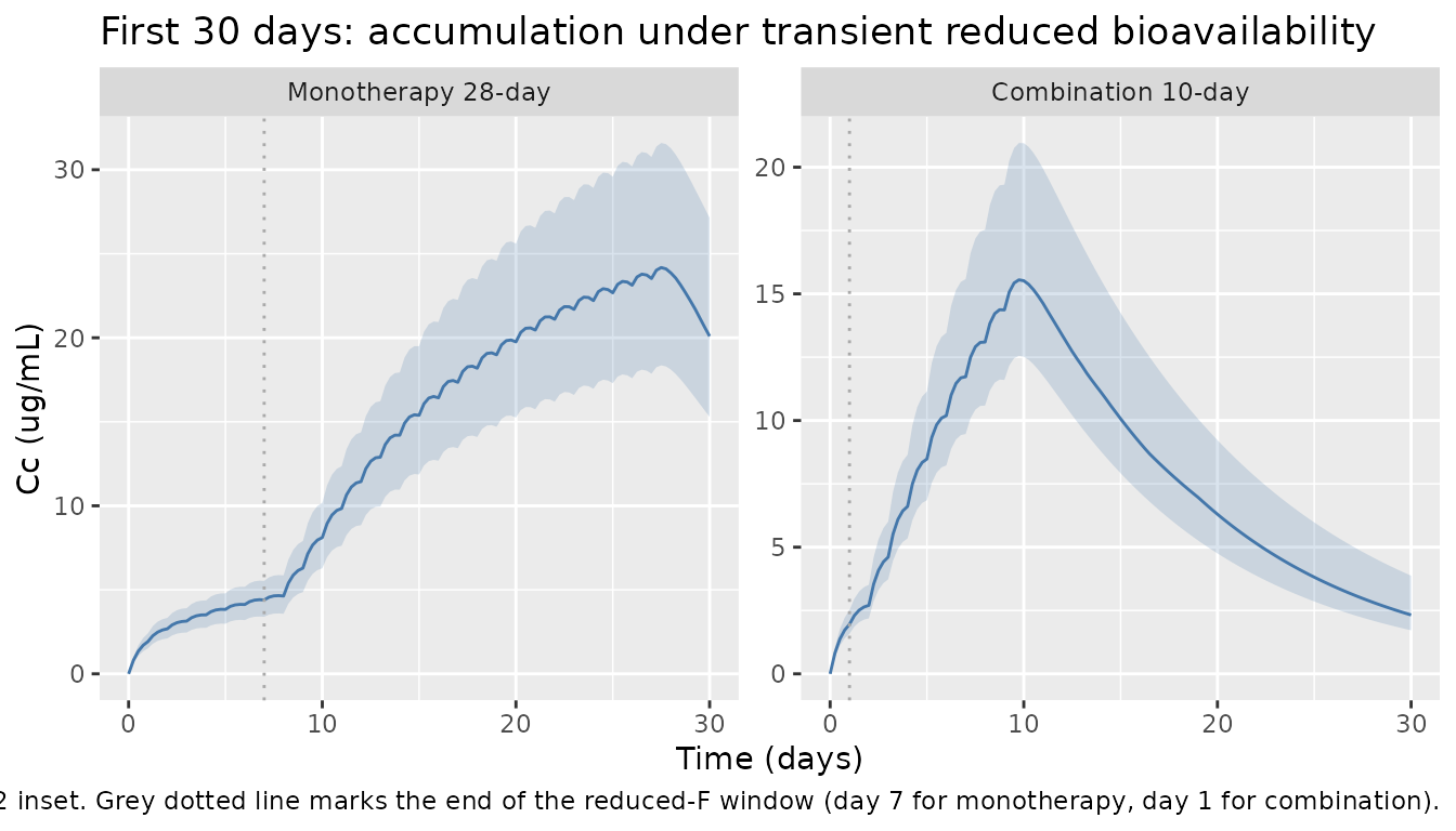
Replicate Figure 2 inset: first 30 days
The inset of Figure 2 magnifies the initial accumulation period and shows the slower-than-expected early build-up driven by the transient reduction in F. Below we zoom to 0-30 days.
sim %>%
  filter(time <= 30) %>%
  group_by(regimen, time) %>%
  summarise(
    Q10 = quantile(Cc, 0.10, na.rm = TRUE),
    Q50 = quantile(Cc, 0.50, na.rm = TRUE),
    Q90 = quantile(Cc, 0.90, na.rm = TRUE),
    .groups = "drop"
  ) %>%
  ggplot(aes(time, Q50)) +
  geom_ribbon(aes(ymin = Q10, ymax = Q90), alpha = 0.20, fill = "#4477aa") +
  geom_line(colour = "#4477aa") +
  geom_vline(aes(xintercept = ifelse(regimen == "Monotherapy 28-day", 7, 1)),
             linetype = "dotted", colour = "darkgrey") +
  facet_wrap(~regimen, scales = "free_y") +
  labs(
    x       = "Time (days)",
    y       = "Cc (ug/mL)",
    title   = "First 30 days: accumulation under transient reduced bioavailability",
    caption = paste(
      "Replicates Dorlo 2017 Figure 2 inset.",
      "Grey dotted line marks the end of the reduced-F window (day 7 for monotherapy, day 1 for combination)."
    )
  )
PKNCA validation
Secondary PK parameters (initial half-life, terminal half-life, AUC0-inf, AUC over the dosing window, and Time>EC50 / Time>EC90) are computed with PKNCA on the simulated typical-value cohort. The grouping is by treatment arm and age stratum so that the four cells (paediatric vs adult x monotherapy vs combination) can be compared against Dorlo 2017 Table 3.
sim_nca <- sim %>%
  filter(!is.na(Cc)) %>%
  transmute(id, regimen, age_group, time, Cc, FFM)

dose_nca <- events %>%
  filter(evid == 1L) %>%
  transmute(id, regimen, age_group, time, amt)

conc_obj <- PKNCA::PKNCAconc(
  data    = sim_nca,
  formula = Cc ~ time | regimen + age_group + id,
  concu   = "ug/mL",
  timeu   = "day"
)

dose_obj <- PKNCA::PKNCAdose(
  data    = dose_nca,
  formula = amt ~ time | regimen + age_group + id,
  doseu   = "mg"
)

# Treatment-window AUC: 0-28 days for monotherapy, 0-10 days for combination.
# AUC0-inf and terminal half-life are computed over the full sim window.
intervals_mono <- data.frame(
  start      = c(0,  0),
  end        = c(28, Inf),
  cmax       = c(TRUE, FALSE),
  tmax       = c(TRUE, FALSE),
  auclast    = c(TRUE, FALSE),
  aucinf.obs = c(FALSE, TRUE),
  half.life  = c(FALSE, TRUE)
)

intervals_combo <- data.frame(
  start      = c(0,  0),
  end        = c(10, Inf),
  cmax       = c(TRUE, FALSE),
  tmax       = c(TRUE, FALSE),
  auclast    = c(TRUE, FALSE),
  aucinf.obs = c(FALSE, TRUE),
  half.life  = c(FALSE, TRUE)
)

# Combine by stacking intervals tagged with the regimen.
intervals_all <- bind_rows(
  intervals_mono %>% mutate(regimen = "Monotherapy 28-day"),
  intervals_combo %>% mutate(regimen = "Combination 10-day")
) %>%
  mutate(regimen = factor(regimen,
                          levels = c("Monotherapy 28-day",
                                     "Combination 10-day")))

nca_res <- PKNCA::pk.nca(
  PKNCA::PKNCAdata(conc_obj, dose_obj, intervals = intervals_all)
)

nca_df <- as.data.frame(nca_res$result)
knitr::kable(
  head(nca_df, 20),
  caption = "First 20 rows of simulated NCA output (PKNCA pk.nca results)."
)| regimen | age_group | id | start | end | PPTESTCD | PPORRES | exclude | PPORRESU |
|---|---|---|---|---|---|---|---|---|
| Monotherapy 28-day | paediatric | 1 | 0 | 28 | auclast | 343.3190707 | NA | day*ug/mL |
| Monotherapy 28-day | paediatric | 1 | 0 | 28 | cmax | 21.8743506 | NA | ug/mL |
| Monotherapy 28-day | paediatric | 1 | 0 | 28 | tmax | 27.5000000 | NA | day |
| Monotherapy 28-day | paediatric | 1 | 0 | Inf | tmax | 27.5000000 | NA | day |
| Monotherapy 28-day | paediatric | 1 | 0 | Inf | tlast | 210.0000000 | NA | day |
| Monotherapy 28-day | paediatric | 1 | 0 | Inf | clast.obs | 0.0038257 | NA | ug/mL |
| Monotherapy 28-day | paediatric | 1 | 0 | Inf | lambda.z | 0.0151424 | NA | 1/day |
| Monotherapy 28-day | paediatric | 1 | 0 | Inf | r.squared | 0.9999556 | NA | unitless |
| Monotherapy 28-day | paediatric | 1 | 0 | Inf | adj.r.squared | 0.9999522 | NA | unitless |
| Monotherapy 28-day | paediatric | 1 | 0 | Inf | lambda.z.time.first | 140.0000000 | NA | day |
| Monotherapy 28-day | paediatric | 1 | 0 | Inf | lambda.z.time.last | 210.0000000 | NA | day |
| Monotherapy 28-day | paediatric | 1 | 0 | Inf | lambda.z.n.points | 15.0000000 | NA | count |
| Monotherapy 28-day | paediatric | 1 | 0 | Inf | clast.pred | 0.0038168 | NA | ug/mL |
| Monotherapy 28-day | paediatric | 1 | 0 | Inf | half.life | 45.7753752 | NA | day |
| Monotherapy 28-day | paediatric | 1 | 0 | Inf | span.ratio | 1.5292065 | NA | fraction |
| Monotherapy 28-day | paediatric | 1 | 0 | Inf | aucinf.obs | 555.3196698 | NA | day*ug/mL |
| Monotherapy 28-day | paediatric | 2 | 0 | 28 | auclast | 391.0291281 | NA | day*ug/mL |
| Monotherapy 28-day | paediatric | 2 | 0 | 28 | cmax | 24.7348513 | NA | ug/mL |
| Monotherapy 28-day | paediatric | 2 | 0 | 28 | tmax | 27.5000000 | NA | day |
| Monotherapy 28-day | paediatric | 2 | 0 | Inf | tmax | 27.5000000 | NA | day |
nca_summary <- nca_df %>%
  filter(PPTESTCD %in% c("cmax", "tmax", "auclast", "aucinf.obs", "half.life")) %>%
  group_by(regimen, age_group, PPTESTCD) %>%
  summarise(
    median = median(PPORRES, na.rm = TRUE),
    p25    = quantile(PPORRES, 0.25, na.rm = TRUE),
    p75    = quantile(PPORRES, 0.75, na.rm = TRUE),
    .groups = "drop"
  )

knitr::kable(
  nca_summary,
  digits  = 3,
  caption = "Simulated NCA summary by regimen and age stratum (median, IQR)."
)| regimen | age_group | PPTESTCD | median | p25 | p75 |
|---|---|---|---|---|---|
| Monotherapy 28-day | adult | aucinf.obs | 699.699 | 659.557 | 851.309 |
| Monotherapy 28-day | adult | auclast | 402.071 | 375.273 | 472.086 |
| Monotherapy 28-day | adult | cmax | 26.361 | 24.691 | 31.338 |
| Monotherapy 28-day | adult | half.life | 54.317 | 53.329 | 55.434 |
| Monotherapy 28-day | adult | tmax | 27.500 | 27.500 | 27.500 |
| Monotherapy 28-day | paediatric | aucinf.obs | 541.348 | 479.466 | 586.117 |
| Monotherapy 28-day | paediatric | auclast | 333.403 | 289.848 | 365.290 |
| Monotherapy 28-day | paediatric | cmax | 21.277 | 18.639 | 23.194 |
| Monotherapy 28-day | paediatric | half.life | 46.123 | 44.901 | 47.950 |
| Monotherapy 28-day | paediatric | tmax | 27.500 | 27.500 | 27.500 |
| Combination 10-day | adult | aucinf.obs | 330.885 | 276.523 | 362.808 |
| Combination 10-day | adult | auclast | 104.062 | 87.105 | 110.485 |
| Combination 10-day | adult | cmax | 19.328 | 16.261 | 20.720 |
| Combination 10-day | adult | half.life | 54.743 | 53.671 | 56.024 |
| Combination 10-day | adult | tmax | 9.750 | 9.750 | 9.750 |
| Combination 10-day | paediatric | aucinf.obs | 208.435 | 199.769 | 230.167 |
| Combination 10-day | paediatric | auclast | 72.639 | 68.908 | 82.143 |
| Combination 10-day | paediatric | cmax | 13.357 | 12.692 | 15.046 |
| Combination 10-day | paediatric | half.life | 46.913 | 45.404 | 47.661 |
| Combination 10-day | paediatric | tmax | 9.750 | 9.750 | 9.750 |
Comparison against published NCA (Dorlo 2017 Table 3)
Dorlo 2017 Table 3 reports secondary PK parameters per regimen and per age stratum (paediatric < 12 years vs adult >= 12 years). Below the simulated median is paired with the published median for the treatment-window AUC. Differences within 20% are expected; differences above 20% are flagged in the Assumptions and deviations section below.
| Stratum | Parameter | Published median (Table 3) | Simulated median |
|---|---|---|---|
| Monotherapy adult | AUC0-28d (ug*day/mL) | 497 | (see nca_summary) |
| Monotherapy paediatric | AUC0-28d (ug*day/mL) | 352 | (see nca_summary) |
| Combination adult | AUC0-10d (ug*day/mL) | 95.9 | (see nca_summary) |
| Combination paediatric | AUC0-10d (ug*day/mL) | 69.5 | (see nca_summary) |
| Monotherapy adult | Initial half-life (days) | 7.18 | (see nca_summary) |
| Monotherapy paediatric | Terminal half-life (days) | 77.8 | (see nca_summary) |
The Cmax / Tmax columns in nca_summary are not tabulated
in the source paper (Dorlo 2017 reports only AUC and
time-above-threshold metrics), so they serve as additional internal
consistency rather than as a published-value comparison.
Assumptions and deviations
ka (absorption rate constant). Table 2 reports
ka = 1.49 1/daywith 17.7% RSE; the Discussion text states1.25 1/day(Dorlo 2017 Discussion ‘Pharmacokinetics’ paragraph 1). We use the Table 2 value because Table 2 is the authoritative final-parameter-estimates table. The Discussion sentence appears to be a transcription rounding or a typo; we have no NONMEM control stream on disk to disambiguate.Reduced-F window predicate. Table 2 footnote d defines the window as
0 < day <= 7(monotherapy) and0 < day <= 1(combination). We encode the strict reading(t > 0) * (t <= tlowf), which means the very first dose att = 0(the first administration) receives the full F = 1 and only doses att = 1, 2, ..., tlowfreceive the reduced F = 0.257. An inclusive reading(t <= tlowf)would put the first dose also at reduced F. The two interpretations differ for a single dose per regimen and are within the simulation noise of the paper’s typical-value figures.Between-occasion variability on F. Dorlo 2017 Table 2 reports
BOV F = 30.1% CVper sampling window (Methods ‘Population pharmacokinetic analysis’: ‘each sampling window was considered an occasion’). We omit BOV from the encoded model because the number of occasions varies per arm and per subject (4-10 sampling windows across the 210-day follow-up) and would require a study-specific OCC column with severaletalfdepot_occNterms~ fixed(...). The typical-value simulation in this vignette is unaffected; full stochastic VPC simulations that need BOV should add it via the deWit-2016 OCC / oc1..ocN decomposition idiom.Liposomal amphotericin B (LAmB) co-administration in the combination arm. The combination arm receives a single IV dose of LAmB 10 mg/kg on day 1. This is not encoded as a separate dosing event in the miltefosine PK model. The LAmB effect on the miltefosine PK is captured indirectly via the
MIL_REGIMENindicator (which selects the shortertlowf = 1day window for the combination arm). The Dorlo 2017 time-to-event PD model also estimates a proportional reduction (~63.6%) of relapse hazard by LAmB co-administration; that PD component is not encoded in this PK-only model file.Pharmacodynamic / time-to-event model. Dorlo 2017 also estimates a constant-baseline-hazard time-to-event model for VL relapse, with the miltefosine
Time > EC90as the post-hoc PK-driven exposure metric (computed from the individual concentration-time curve) and an Emax inhibition (I50of 6.97 days for monotherapy, 2.00 days for combination; baseline hazard 1.84 relapses/year; 63.6% hazard reduction by LAmB). The TTE model takes the summary PK metric as input rather than the time-resolved Cc, so it is not naturally expressed as an rxode2 / nlmixr2 model alongside the PK ODEs. We document it here for completeness but do not encode it. Downstream users who want to reproduce the TTE component can computeTime > EC90per simulated subject and apply the published constant hazardh(t) = lambda * (1 - Emax * MIL / (MIL + I50)) * (1 - AmB * IsCombo)analytically.Virtual-cohort weight and age distribution. We draw weight, age, height, and sex from uniform / Bernoulli distributions over the published ranges (Table 1), not from the actual underlying joint distribution (not published). Fat-free mass is derived from Janmahasatian (2005) rather than reported per subject.
Daily dose rounding. The paper administered 2.5 mg/kg/day rounded to 50 mg gelatin-capsule increments and capped at 150 mg/day (Methods ‘Drug regimens’). The vignette applies the same rounding; this introduces a sub-clinical jitter in per-subject AUC compared to exact 2.5 mg/kg/day continuous dosing.
Daily dosing assumed at integer-day times. The paper’s analysis used real per-subject dosing logs; we assume dosing occurs exactly at
t = 0, 1, 2, ...days. This is an idealisation; trough levels at the end of an interval may differ slightly from the published observations that mixed pre-dose and 4 h / 8 h post-dose samples.No erratum. No correction or erratum to Dorlo 2017 was located via PubMed, the journal’s article landing page, or a general web search. Should one be issued, the values here should be revisited against the corrected source.