Lenalidomide (Kim 2026)
Source:vignettes/articles/Kim_2026_lenalidomide.Rmd
Kim_2026_lenalidomide.RmdModel and source
- Citation: Kim H, Park S-S, Choi S, Han S, Han S, Lee Y, Lee JH, Kim D, Kim H, Yang S, Shugg T, Chung EK. Population Pharmacokinetics and Model-Informed Precision Dosing of Lenalidomide Incorporating Total and Unbound Plasma Concentrations in Renally Impaired Patients with Multiple Myeloma. Drug Des Devel Ther. 2026;20. doi:10.2147/DDDT.S605741
- Description: Two-compartment oral population PK model with first-order absorption (Ka fixed), first-order elimination and linear (concentration-independent) plasma protein binding for lenalidomide in Korean adults with multiple myeloma spanning normal renal function to severe renal impairment, fitted simultaneously to total and unbound plasma concentrations (Kim 2026). The structural parameters are apparent UNBOUND parameters: CL/F depends on CKD-EPI 2021 eGFR (exponential, centred at 46.92 mL/min/1.73 m^2) and on body surface area (linear, centred at 1.64 m^2); V1/F depends on body surface area (exponential). The total concentration is the unbound concentration divided by a constant unbound fraction of 0.614.
- Article: https://doi.org/10.2147/DDDT.S605741 (open access, PMC13186237)
Kim et al. fitted total and unbound plasma lenalidomide concentrations simultaneously in multiple myeloma patients whose renal function ranged from normal to severe impairment. The structural parameters are apparent unbound parameters; the total concentration follows from a constant unbound fraction (linear protein binding, selected over a saturable Bmax/KD form). Renal function (CKD-EPI 2021 eGFR) and body surface area were the only retained covariates.
Population
Thirty Korean adults with multiple myeloma (Seoul St. Mary’s Hospital) who were starting lenalidomide-based maintenance therapy, stratified by CKD-EPI 2021 eGFR into severe renal impairment (n = 11, eGFR < 30 mL/min/1.73 m^2), moderate renal impairment (n = 11, 30 to < 60) and a control group (n = 8, >= 60). Median age 68 years (47-84), 40% male, median weight 62 kg (47-86), median BSA 1.64 m^2 (1.41-2.01), median eGFR 47 (11.1-94.7) mL/min/1.73 m^2. Doses were 5, 7.5 or 10 mg once daily (Kim 2026 Table 1). Serial samples were drawn pre-dose and 2, 4, 8, 12 and 24 h after the dose on day 3 of cycle 1; 171 total and 174 unbound concentrations entered the analysis.
The same information is available programmatically via
readModelDb("Kim_2026_lenalidomide")()$population.
Source trace
| Equation / parameter | Value | Source location |
|---|---|---|
lka (fixed) |
log(1.16) 1/h | Table 3 theta-Ka (N/E); Results ‘Structural Base Model Building’ |
lcl |
log(8.52) L/h | Table 3 theta-CL/F |
lvc |
log(48.8) L | Table 3 theta-V1/F |
lq |
log(8.05) L/h | Table 3 theta-Q/F |
lvp |
log(21.2) L | Table 3 theta-V2/F |
lfu |
log(0.614) | Table 3 theta-Fu = 61.4% |
e_crcl_cl |
0.0131 | Table 3 theta-CLeGFR |
e_bsa_cl |
1.1 | Table 3 theta-CLBSA |
e_bsa_vc |
1.16 | Table 3 theta-V1BSA |
etalcl |
0.189^2 | Table 3 omega CL/F = 18.9% |
etalvc |
0.308^2 | Table 3 omega V1/F = 30.8% |
propSd, addSd
|
0.126, 2.19 ng/mL | Table 3 sigma total-proportional / total-additive |
propSd_Cu, addSd_Cu
|
0.125, 1.11 ng/mL | Table 3 sigma unbound-proportional / unbound-additive |
cl, vc covariate equations |
n/a | Results, final-model equations (page 10); CL/F form see Assumptions |
Cc <- Cu / fu |
n/a | Methods, ‘Linear Protein Binding’ equation (page 5) |
| Two-compartment ODEs, first-order absorption | n/a | Results ‘Structural Base Model Building’ |
Model structure check
mod <- readModelDb("Kim_2026_lenalidomide")
ui <- rxode2::rxode(mod)
#> ℹ parameter labels from comments will be replaced by 'label()'
th <- ui$theta

# Typical values at the covariate references (eGFR 46.92, BSA 1.64) are the
# Table 3 estimates.
stopifnot(
  abs(exp(th[["lcl"]]) - 8.52) < 1e-10,
  abs(exp(th[["lvc"]]) - 48.8) < 1e-10,
  abs(exp(th[["lfu"]]) - 0.614) < 1e-10
)
Virtual cohort
Individual covariates are not published. Each renal stratum draws eGFR and BSA independently from a triangular distribution spanning the stratum’s Table 1 range with its mode at the stratum median. The dose mix within each stratum follows Table 1 (severe: 9/11 on 7.5 mg, 2/11 on 10 mg; moderate: 3/11 on 5 mg, 2/11 on 7.5 mg, 6/11 on 10 mg; control: 2/8 on 5 mg, 6/8 on 10 mg). Doses are given once daily at 0, 24 and 48 h and the day-3 interval (48-72 h) is sampled, as in the study.
set.seed(2026)

rtri <- function(n, lo, hi, mode) {
  u <- stats::runif(n)
  f <- (mode - lo) / (hi - lo)
  ifelse(
    u < f,
    lo + sqrt(u * (hi - lo) * (mode - lo)),
    hi - sqrt((1 - u) * (hi - lo) * (hi - mode))
  )
}

# Table 1, median (range) per stratum
strata <- tibble::tribble(
  ~stratum,      ~egfr_lo, ~egfr_hi, ~egfr_med, ~bsa_lo, ~bsa_hi, ~bsa_med,
  "Severe RI",   11.1,     28.6,     25.2,      1.49,    1.84,    1.60,
  "Moderate RI", 31.3,     59.9,     52.1,      1.48,    2.01,    1.65,
  "Control",     60.5,     94.7,     77.4,      1.41,    1.91,    1.75
)
dose_mix <- list(
  "Severe RI"   = c(`7.5` = 9, `10` = 2),
  "Moderate RI" = c(`5` = 3, `7.5` = 2, `10` = 6),
  "Control"     = c(`5` = 2, `10` = 6)
)

n_per_stratum <- 200L

make_stratum <- function(s, id_offset) {
  row <- strata[strata$stratum == s, ]
  mix <- dose_mix[[s]]
  n_by_dose <- round(n_per_stratum * mix / sum(mix))
  n_by_dose[length(n_by_dose)] <- n_per_stratum - sum(n_by_dose[-length(n_by_dose)])
  tibble(
    id = id_offset + seq_len(n_per_stratum),
    stratum = s,
    dose = rep(as.numeric(names(mix)), times = n_by_dose),
    CRCL = rtri(n_per_stratum, row$egfr_lo, row$egfr_hi, row$egfr_med),
    BSA = rtri(n_per_stratum, row$bsa_lo, row$bsa_hi, row$bsa_med)
  )
}

subjects <- bind_rows(
  make_stratum("Severe RI", 0L),
  make_stratum("Moderate RI", 200L),
  make_stratum("Control", 400L)
)

# Paper sampling schedule on day 3 (Methods) plus a dense grid for plotting
obs_times <- sort(unique(c(48 + c(0, 2, 4, 8, 12, 24), seq(48, 72, by = 0.5))))

doses <- subjects |>
  tidyr::crossing(time = c(0, 24, 48)) |>
  mutate(evid = 1L, amt = dose, cmt = "depot", dvid = NA_integer_)
# Observation rows carry dvid and no compartment: both Cc (dvid 1) and Cu are
# returned as columns on every observation row.
obs <- subjects |>
  tidyr::crossing(time = obs_times) |>
  mutate(evid = 0L, amt = NA_real_, cmt = NA_character_, dvid = 1L)
events <- bind_rows(doses, obs) |>
  select(id, time, evid, amt, cmt, dvid, CRCL, BSA, stratum, dose) |>
  arrange(id, time, desc(evid))
stopifnot(!anyDuplicated(unique(events[, c("id", "time", "evid")])))
Simulation
sim <- rxode2::rxSolve(mod, events = events, keep = c("stratum", "dose", "CRCL", "BSA")) |>
  as.data.frame()
#> ℹ parameter labels from comments will be replaced by 'label()'
stopifnot(all(c("Cc", "Cu") %in% names(sim)))
# Linear binding: total / unbound is the constant 1 / fu everywhere.
stopifnot(max(abs(sim$Cu / sim$Cc - 0.614), na.rm = TRUE) < 1e-8)
sim$stratum <- factor(sim$stratum, levels = strata$stratum)
Concentration-time profiles (Figures 1 and 4)
sim |>
  select(id, time, stratum, Total = Cc, Unbound = Cu) |>
  pivot_longer(c(Total, Unbound), names_to = "analyte", values_to = "conc") |>
  mutate(tad = time - 48) |>
  group_by(stratum, analyte, tad) |>
  summarise(
    Q05 = quantile(conc, 0.05), Q50 = median(conc), Q95 = quantile(conc, 0.95),
    .groups = "drop"
  ) |>
  ggplot(aes(tad, Q50, colour = stratum, fill = stratum)) +
  geom_ribbon(aes(ymin = Q05, ymax = Q95), alpha = 0.15, colour = NA) +
  geom_line() +
  facet_wrap(~analyte) +
  labs(
    x = "Time after dose on day 3 (h)", y = "Lenalidomide (ng/mL)",
    colour = NULL, fill = NULL,
    caption = "Median and 90% interval; compare Figures 1 and 4 of Kim 2026."
  ) +
  theme(legend.position = "bottom")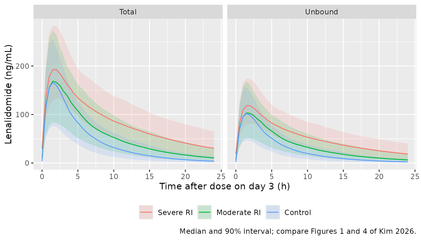
PKNCA validation
NCA uses the study’s own sampling schedule (pre-dose, 2, 4, 8, 12 and 24 h on day 3), so Tmax can only fall on a sampled time, exactly as in Table 2.
run_nca <- function(sim, conc_col) {
  conc <- sim |>
    filter(time %in% (48 + c(0, 2, 4, 8, 12, 24))) |>
    mutate(conc = .data[[conc_col]], stratum = as.character(stratum)) |>
    filter(!is.na(conc)) |>
    select(id, time, conc, stratum)
  dose_df <- events |>
    filter(evid == 1L) |>
    select(id, time, amt, stratum)
  conc_obj <- PKNCA::PKNCAconc(conc, conc ~ time | stratum + id)
  dose_obj <- PKNCA::PKNCAdose(dose_df, amt ~ time | stratum + id)
  intervals <- data.frame(
    start = 48, end = 72,
    cmax = TRUE, tmax = TRUE, auclast = TRUE, half.life = TRUE
  )
  PKNCA::pk.nca(PKNCA::PKNCAdata(conc_obj, dose_obj, intervals = intervals))
}

nca_total <- run_nca(sim, "Cc")
nca_unbound <- run_nca(sim, "Cu")

# Table 2 reports mean +/- SD, so the simulation is summarised by the mean too.
mean_by_stratum <- function(res) {
  as.data.frame(res) |>
    filter(PPTESTCD %in% c("cmax", "tmax", "auclast", "half.life")) |>
    group_by(stratum, PPTESTCD) |>
    summarise(PPORRES = mean(PPORRES, na.rm = TRUE), .groups = "drop") |>
    pivot_wider(names_from = PPTESTCD, values_from = PPORRES)
}

# Kim 2026 Table 2 (mean)
published_total <- tibble::tribble(
  ~stratum,      ~cmax, ~tmax, ~auclast, ~half.life,
  "Severe RI",   227.0, 1.71,  2469.5,   9.80,
  "Moderate RI", 181.7, 2.05,  1531.0,   5.69,
  "Control",     196.2, 1.69,  1263.2,   4.17
)
published_unbound <- tibble::tribble(
  ~stratum,      ~cmax, ~tmax, ~auclast, ~half.life,
  "Severe RI",   143.7, 1.71,  1532.9,   10.04,
  "Moderate RI", 111.9, 2.05,  933.5,    5.55,
  "Control",     122.7, 1.69,  767.6,    3.91
)

nca_units <- c(cmax = "ng/mL", tmax = "h", auclast = "ng*h/mL", half.life = "h")
cmp_total <- nlmixr2lib::ncaComparisonTable(
  simulated = mean_by_stratum(nca_total), reference = published_total,
  by = "stratum", units = nca_units
)
cmp_unbound <- nlmixr2lib::ncaComparisonTable(
  simulated = mean_by_stratum(nca_unbound), reference = published_unbound,
  by = "stratum", units = nca_units
)
cmp <- bind_rows(
  cmp_total |> mutate(Analyte = "Total", .before = 1),
  cmp_unbound |> mutate(Analyte = "Unbound", .before = 1)
)
knitr::kable(
  cmp,
  caption = "Simulated vs. Kim 2026 Table 2 NCA (means; AUC0-24 shown as AUClast over the day-3 interval). * differs by >20%."
)| Analyte | NCA parameter | stratum | Reference | Simulated | % diff |
|---|---|---|---|---|---|
| Total | Cmax (ng/mL) | Severe RI | 227 | 196 | -13.6% |
| Total | Cmax (ng/mL) | Moderate RI | 182 | 168 | -7.4% |
| Total | Cmax (ng/mL) | Control | 196 | 156 | -20.7%* |
| Total | Tmax (h) | Severe RI | 1.71 | 2 | +17.0% |
| Total | Tmax (h) | Moderate RI | 2.05 | 2 | -2.4% |
| Total | Tmax (h) | Control | 1.69 | 2 | +18.3% |
| Total | AUClast (ng*h/mL) | Severe RI | 2470 | 2080 | -15.6% |
| Total | AUClast (ng*h/mL) | Moderate RI | 1530 | 1370 | -10.2% |
| Total | AUClast (ng*h/mL) | Control | 1260 | 989 | -21.7%* |
| Total | t½ (h) | Severe RI | 9.8 | 9.31 | -5.0% |
| Total | t½ (h) | Moderate RI | 5.69 | 6.37 | +12.0% |
| Total | t½ (h) | Control | 4.17 | 4.69 | +12.4% |
| Unbound | Cmax (ng/mL) | Severe RI | 144 | 120 | -16.2% |
| Unbound | Cmax (ng/mL) | Moderate RI | 112 | 103 | -7.7% |
| Unbound | Cmax (ng/mL) | Control | 123 | 95.6 | -22.1%* |
| Unbound | Tmax (h) | Severe RI | 1.71 | 2 | +17.0% |
| Unbound | Tmax (h) | Moderate RI | 2.05 | 2 | -2.4% |
| Unbound | Tmax (h) | Control | 1.69 | 2 | +18.3% |
| Unbound | AUClast (ng*h/mL) | Severe RI | 1530 | 1280 | -16.5% |
| Unbound | AUClast (ng*h/mL) | Moderate RI | 934 | 844 | -9.6% |
| Unbound | AUClast (ng*h/mL) | Control | 768 | 607 | -20.9%* |
| Unbound | t½ (h) | Severe RI | 10 | 9.31 | -7.3% |
| Unbound | t½ (h) | Moderate RI | 5.55 | 6.37 | +14.8% |
| Unbound | t½ (h) | Control | 3.91 | 4.69 | +19.9% |
auc_cmp <- mean_by_stratum(nca_total) |>
  inner_join(published_total, by = "stratum", suffix = c("_sim", "_pub")) |>
  mutate(pct = 100 * (auclast_sim / auclast_pub - 1))
stopifnot(nrow(auc_cmp) == 3L)
# The model sits about 15% below the observed means in every stratum (see
# below); across seeds and thread counts the mean of the three differences was
# -15 to -17% and single strata ranged -6 to -24%. A mis-transcribed fu, a
# swapped CL/V or a unit slip moves AUC by 40% or more and still fails here.
stopifnot(
  abs(mean(auc_cmp$pct)) < 25,
  all(abs(auc_cmp$pct) < 35)
)
Simulated day-3 AUC0-24 and Cmax fall below the observed Table 2 means in all three strata, by about 10-20% (most in the control and severe-RI strata), while the half-lives agree within 20%. The observed means come from only 8-11 patients each with coefficients of variation of 25-60% (the control-stratum AUC is 1,263 +/- 758 ng*h/mL), so each observed mean carries a standard error of roughly 8-20%; the shortfall is nonetheless in the same direction in every stratum. The paper’s own Figure 6 points the same way: fitting a typical unbound clearance at BSA 1.64 m^2 to its 84 PTA cells gives about 5.5 L/h for the severe-RI stratum, lower than this model’s 6.1-6.4 L/h at that stratum’s mean and median eGFR (see the next section). The parameters are used as published; they have not been adjusted to close the gap. Tmax lands on the 2-h sample because the schedule has no earlier post-dose time, which is also why the observed Tmax values sit close to 2 h.
Probability of target attainment (Figure 6)
Kim 2026 simulated steady-state total AUC0-24 for virtual patients
with BSA fixed at 1.4 to 2.0 m^2 and eGFR drawn from each renal stratum,
and reported the fraction falling within the target 1,615.5-2,692.5
ng*h/mL. At steady state AUC0-24 = dose / (CL/F x fu) for this linear
model, so each subject’s AUC is computed from its individual
cl and fu; the chunk below checks that
identity against an ODE solve.
pta_doses <- c(5, 7.5, 10, 15, 20, 25)
pta_bsa <- seq(1.4, 2.0, by = 0.1)
n_cell <- 200L

pta_subjects <- tidyr::crossing(
  stratum = c("Severe RI", "Moderate RI"), BSA = pta_bsa, rep = seq_len(n_cell)
) |>
  mutate(id = seq_len(n()))
pta_subjects$CRCL <- ifelse(
  pta_subjects$stratum == "Severe RI",
  rtri(nrow(pta_subjects), 11.1, 28.6, 25.2),
  rtri(nrow(pta_subjects), 31.3, 59.9, 52.1)
)

pta_ev <- pta_subjects |>
  mutate(time = 0, evid = 0L, amt = NA_real_, cmt = NA_character_, dvid = 1L)
pta_par <- rxode2::rxSolve(mod, events = pta_ev, keep = c("stratum", "BSA", "CRCL")) |>
  as.data.frame() |>
  select(id, stratum, BSA, CRCL, cl, fu)

# Closed-form AUC0-24,ss against a 14-day ODE solve for a few subjects.
chk_ids <- pta_par$id[seq(1, nrow(pta_par), length.out = 6)]
chk_ev <- pta_subjects |>
  filter(id %in% chk_ids) |>
  tidyr::crossing(time = seq(0, 312, by = 24)) |>
  mutate(evid = 1L, amt = 10, cmt = "depot", dvid = NA_integer_) |>
  bind_rows(
    pta_subjects |>
      filter(id %in% chk_ids) |>
      tidyr::crossing(time = seq(312, 336, by = 0.02)) |>
      mutate(evid = 0L, amt = NA_real_, cmt = NA_character_, dvid = 1L)
  ) |>
  arrange(id, time, desc(evid))
# Typical-value solve with these subjects' covariates; the identity is checked
# against the cl and fu of the same solve.
chk_sim <- rxode2::rxSolve(
  mod, events = chk_ev, omega = NA, rtol = 1e-10, atol = 1e-12
) |>
  as.data.frame()
#> Warning: multi-subject simulation without without 'omega'
chk_auc <- chk_sim |>
  group_by(id) |>
  summarise(
    auc_ode = sum(diff(time) * (head(Cc, -1) + tail(Cc, -1)) / 2),
    cl = first(cl), fu = first(fu), .groups = "drop"
  ) |>
  mutate(auc_closed = 10 * 1000 / (cl * fu))
# Trapezoid on a 0.02 h grid after 13 daily doses; measured ~1e-4 relative.
stopifnot(max(abs(chk_auc$auc_ode / chk_auc$auc_closed - 1)) < 0.005)
# Kim 2026 Figure 6 cell labels, rows = dose (5 ... 25 mg), columns = BSA 1.4 ... 2.0
paper_pta <- list(
  "Severe RI" = rbind(
    c(69.6, 58.9, 41.6, 25.9, 15.1, 8.0, 4.2),
    c(28.4, 50.8, 66.8, 70.7, 64.3, 54.0, 42.5),
    c(4.1, 13.5, 28.6, 45.9, 59.5, 67.6, 70.0),
    c(0.0, 0.2, 1.2, 3.6, 8.8, 16.2, 26.1),
    c(0.0, 0.0, 0.0, 0.1, 0.4, 1.4, 3.1),
    c(0.0, 0.0, 0.0, 0.0, 0.0, 0.1, 0.2)
  ),
  "Moderate RI" = rbind(
    c(28.0, 14.2, 6.2, 2.6, 1.2, 0.5, 0.1),
    c(63.8, 56.0, 41.2, 29.0, 19.0, 11.7, 7.1),
    c(45.1, 60.8, 65.5, 60.4, 50.8, 40.0, 30.6),
    c(4.6, 13.8, 28.1, 44.4, 56.0, 63.2, 65.9),
    c(0.2, 1.1, 3.9, 9.9, 19.0, 30.4, 41.3),
    c(0.0, 0.0, 0.2, 1.0, 3.6, 7.6, 14.2)
  )
)
paper_long <- bind_rows(lapply(names(paper_pta), function(s) {
  m <- paper_pta[[s]]
  tibble(
    stratum = s,
    dose = rep(pta_doses, times = length(pta_bsa)),
    BSA = rep(pta_bsa, each = length(pta_doses)),
    pta_paper = as.vector(m)
  )
}))

lo <- 1615.5
hi <- 2692.5
bsa_ref <- 1.64
e_bsa <- th[["e_bsa_cl"]]
pta_sim <- pta_par |>
  tidyr::crossing(dose = pta_doses) |>
  mutate(
    # Encoded (linear) form
    auc_linear = dose * 1000 / (cl * fu),
    # Printed form: the same exponential part plus an additive BSA offset
    cl_printed = cl / (1 + e_bsa * (BSA - bsa_ref)) + e_bsa * (BSA - bsa_ref),
    auc_printed = dose * 1000 / (cl_printed * fu)
  ) |>
  group_by(stratum, dose, BSA) |>
  summarise(
    pta_linear = 100 * mean(auc_linear >= lo & auc_linear <= hi),
    pta_printed = 100 * mean(auc_printed >= lo & auc_printed <= hi),
    .groups = "drop"
  ) |>
  mutate(BSA = round(BSA, 1)) |>
  inner_join(paper_long |> mutate(BSA = round(BSA, 1)), by = c("stratum", "dose", "BSA"))
stopifnot(nrow(pta_sim) == 84L)

rmse <- pta_sim |>
  summarise(
    linear = sqrt(mean((pta_linear - pta_paper)^2)),
    printed = sqrt(mean((pta_printed - pta_paper)^2))
  )
knitr::kable(rmse, digits = 1, caption = "RMSE (percentage points) against the 84 Figure 6 cells.")| linear | printed |
|---|---|
| 8.5 | 17.8 |
pta_sim |>
  select(stratum, dose, BSA, `Kim 2026 Figure 6` = pta_paper, `This model` = pta_linear) |>
  pivot_longer(c(`Kim 2026 Figure 6`, `This model`), names_to = "source", values_to = "pta") |>
  mutate(stratum = factor(stratum, levels = c("Severe RI", "Moderate RI"))) |>
  ggplot(aes(factor(BSA), factor(dose), fill = pta)) +
  geom_tile() +
  geom_text(aes(label = sprintf("%.0f", pta)), size = 2.6) +
  facet_grid(stratum ~ source) +
  scale_fill_gradient(low = "white", high = "darkorange", limits = c(0, 100)) +
  labs(x = "BSA (m^2)", y = "Daily dose (mg)", fill = "PTA (%)",
       caption = "Replicates Figure 6 of Kim 2026.")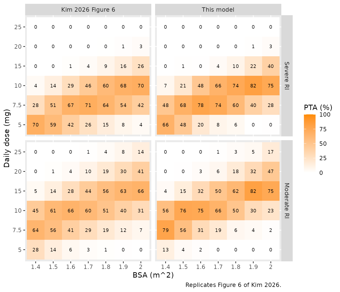
best_dose <- function(df, col) {
  df |>
    group_by(stratum, BSA) |>
    slice_max(.data[[col]], n = 1, with_ties = FALSE) |>
    ungroup() |>
    select(stratum, BSA, dose)
}
best <- inner_join(
  best_dose(pta_sim, "pta_paper"), best_dose(pta_sim, "pta_linear"),
  by = c("stratum", "BSA"), suffix = c("_paper", "_model")
)
edge <- best |> filter(BSA %in% c(1.4, 2.0))
knitr::kable(edge, caption = "Dose with the highest PTA at the edges of the BSA range.")| stratum | BSA | dose_paper | dose_model |
|---|---|---|---|
| Moderate RI | 1.4 | 7.5 | 7.5 |
| Moderate RI | 2.0 | 15.0 | 15.0 |
| Severe RI | 1.4 | 5.0 | 5.0 |
| Severe RI | 2.0 | 10.0 | 10.0 |
stopifnot(
  # The paper's dosing recommendations: at BSA 1.4 the best dose is 5 mg
  # (severe) / 7.5 mg (moderate); at BSA 2.0 it is 10 mg / 15 mg. In this
  # model those winners lead the runner-up by about 20 percentage points,
  # several binomial SEs at 200 subjects per cell.
  all(edge$dose_paper == edge$dose_model),
  # Overall agreement with the 84 cells: RMSE 8.5-9.2 points for the encoded
  # form and 17.4-17.8 for the printed additive form across seeds and thread
  # counts (both computed from the same draws, so the gap is stable).
  rmse$linear < 12,
  rmse$printed > rmse$linear + 4
)
The encoded model reproduces the dose-by-BSA structure of Figure 6: the dose that maximises target attainment rises from 5 to 10 mg (severe RI) and from 7.5 to 15 mg (moderate RI) as BSA goes from 1.4 to 2.0 m^2. The printed additive form gives a nearly flat BSA gradient and about twice the error. The best cell in each stratum reaches about 80% in this model against 70% in the paper, so the published simulation had a wider AUC spread than IIV on CL/F and the sampled eGFR produce here. The paper describes its virtual eGFR only as “eGFR data from our patient cohort”, and its simulated AUC may include residual error; either would widen the spread.
Assumptions and deviations
-
Functional form of the BSA effect on CL/F. The
page-10 final-model equation prints
CL/F = 8.52 * exp[0.0131 * (eGFR - 46.92)] + 1.1 * (BSA - 1.64), with the closing bracket before the BSA term, making it an additive offset of 1.1 L/h per m^2. That form changes CL/F by only about 12% across BSA 1.4-2.0 m^2 and cannot produce the paper’s own Figure 6 or its dosing recommendations, which need about a two-fold change. The maintainers fitted all 84 Figure 6 cells under three readings, each with the same three free parameters (a typical clearance per renal stratum and one log-normal AUC spread): linear* (1 + 1.1 * (BSA - 1.64))gave an RMSE of 1.6 percentage points, exponentialexp[... + 1.1 * (BSA - 1.64)]2.4, and the printed additive form 13.6. The linear form is encoded: it fits best and is the form the Discussion names (“the model that included BSA as a linear covariate on CL/F”). The PTA comparison above repeats the test with this model’s own simulation. - V2/F prints as 21.1 L in the page-10 equation and 21.2 L in Table 3; 21.1 is the bootstrap median, and the Table 3 NONMEM estimate of 21.2 L is used.
- IIV scale. Table 3 reports omega as a percentage under an “omega” (not “omega^2”) header; it is read as the log-scale SD, so the variances are 0.189^2 and 0.308^2. Reading the percentages as CVs instead would change the variances by under 2%.
- eGFR reference. The CL/F equation centres eGFR at 46.92 mL/min/1.73 m^2, slightly different from the Table 1 cohort median of 47; the printed 46.92 is used.
- Virtual covariates. eGFR and BSA are drawn independently from triangular distributions over each stratum’s Table 1 range with the mode at the stratum median. Individual covariates were not published.
- Steady state. The study sampled on day 3 of cycle 1 and analysed the data as steady state; the NCA comparison simulates three daily doses and uses the third interval, as in the study.
- Table 3 labels two residual-error rows “addictive”; they are the additive components.