Canrenone (Suyagh 2012)
Source:vignettes/articles/Suyagh_2012_canrenone.Rmd
Suyagh_2012_canrenone.RmdModel and source
- Citation: Suyagh M, Hawwa AF, Collier PS, Millership JS, Kole P, Millar M, Shields MD, Halliday HL, McElnay JC (2012). Population pharmacokinetic model of canrenone after intravenous administration of potassium canrenoate to paediatric patients. British Journal of Clinical Pharmacology 74(5):864-872.
- Article: https://doi.org/10.1111/j.1365-2125.2012.04257.x
- Description: One-compartment population PK model for canrenone (the
pharmacologically active metabolite of intravenous potassium canrenoate,
K-canrenoate) in 23 paediatric patients receiving K-canrenoate in the
NICU / PICU for management of retained fluids or congestive heart
failure. The K-canrenoate dose compartment (modelled as
depotsince only canrenone is measured) is converted to canrenone at the first-order metabolic transformation ratekf = 5.25 1/h. Canrenone disposition is described by an apparent clearanceCL/F = 11.4 L/hand apparent volumeV/F = 374.2 Lat a reference weight of 70 kg, with bodyweight entering through fixed allometric exponents (0.75 on CL and 1.0 on V). The paper retained no other covariate in the final model.
Population
Twenty-three paediatric patients (15 male, 8 female) admitted to the NICU at the Royal Jubilee Maternity Service, Belfast, or to the medical and intensive care wards at the Royal Belfast Hospital for Sick Children, who received intravenous K-canrenoate as part of routine care for retained fluids (15 of 23, including pulmonary oedema secondary to chronic lung disease) or congestive heart failure (8 of 23). The cohort spans 2 days to 10 years of postnatal age, with median weight 4 kg (range 2.16-28.0 kg) and 20 of 23 subjects younger than 1 year (the other three subjects were 2, 6, and 10 years old). Gestational age at birth ranged 25-41 weeks (median 37 weeks; 2 very preterm, 9 preterm all at 36 weeks, 12 full-term). Baseline characteristics are reported in Suyagh 2012 Table 1.
A total of 101 plasma canrenone concentrations were collected, with 1-8 samples per patient (median 4). Concentrations were determined by HPLC with UV detection (LOQ 25 ng/mL).
The same information is available programmatically via the model’s
population metadata
(readModelDb("Suyagh_2012_canrenone")$population).
Source trace
The per-parameter origin is recorded as an in-file comment next to
each ini() entry in
inst/modeldb/specificDrugs/Suyagh_2012_canrenone.R. The
table below collects the principal entries in one place for review.
| Quantity | Value | Source location |
|---|---|---|
| Canrenone CL/F at WT = 70 kg | 11.4 L/h | Table 3, theta_CL/F final model (RSE 10.3%) |
| Canrenone V/F at WT = 70 kg | 374.2 L | Table 3, theta_V/F final model (RSE 20.04%) |
| K-canrenoate to canrenone rate kf | 5.25 1/h | Table 3, theta_kf final model (RSE 57.84%) |
| Allometric exponent on CL | 0.75 (fixed) | Methods p. 866 + Table 3 final model (theta_1) |
| Allometric exponent on V | 1.0 (fixed) | Methods p. 866 + Table 3 final model (theta_2) |
| Reference weight | 70 kg | Methods p. 866 (allometric scaling normalisation) |
| IIV CL/F | 41.06 % CV | Table 3, omega_CL/F (RSE 44.25%) |
| IIV V/F | 45.76 % CV | Table 3, omega_V/F (RSE 60.06%) |
| Residual error (proportional only) | 34.07 % CV | Table 3, sigma_prop (RSE 23.08%) |
| Structural model: 1-cmt parent + cmt mass | n/a | Methods p. 866 - “one compartment model best described the data”; Figure 1 schematic |
| Typical CL/F at 4 kg | 1.33 L/h | Results p. 868 + abstract |
| Typical V/F at 4 kg | 21.4 L | Results p. 868 + abstract |
| Typical half-life at 4 kg | 11.2 h | Results p. 868 + abstract |
| Typical Tmax | 0.85 h (51 min) | Results - Lactonization, p. 868 |
| Canrenone ke at 4 kg | 0.062 1/h | Results - Lactonization, p. 868 |
| Lactonization t1/2 = ln(2) / kf | 0.13 h (7.8 min) | Results - Lactonization, p. 868 |
Virtual cohort
The original observed concentration-time data are not publicly available. The figures below use a virtual paediatric cohort whose covariate distribution (body weight) approximates the Suyagh 2012 Table 1 demographics: a primary group of neonates and infants under 1 year (most of the cohort) plus a small tail of older paediatric patients (2, 6, 10 years), reflecting the published 23-patient distribution. Body weight is the only covariate retained in the final model.
set.seed(20260613)

# Weight distribution from Suyagh 2012 Table 1:
#   * 20/23 subjects < 1 year, weights 2.16-6.3 kg (cluster around 4 kg)
#   * 1 subject ~ 2 y / ~12 kg
#   * 1 subject ~ 6 y / ~20 kg
#   * 1 subject ~ 10 y / 28 kg
#
# We oversample to N = 100 to give a stable VPC envelope while keeping
# the same relative weight distribution. Doses are scaled to the
# weight band (3.77-70.43 umol K-canrenoate observed in the paper,
# Table 1) so larger children receive larger absolute doses, mimicking
# clinical practice.

n_infants  <- 87L     # < 1 year, weight 2.16-6.3 kg
n_toddler  <-  5L     # ~ 2 years, weight 10-14 kg
n_child    <-  4L     # ~ 6 years, weight 18-22 kg
n_older    <-  4L     # ~ 10 years, weight 26-30 kg
n_subjects <- n_infants + n_toddler + n_child + n_older

wt_infants <- pmin(pmax(rnorm(n_infants, mean = 4, sd = 1.1), 2.16), 6.3)
wt_toddler <- runif(n_toddler, 10, 14)
wt_child   <- runif(n_child,   18, 22)
wt_older   <- runif(n_older,   26, 30)
weights    <- c(wt_infants, wt_toddler, wt_child, wt_older)

# K-canrenoate dose in umol: mg/kg-style scaling, anchored to the
# paper's mean dose (10.06 umol at median 4 kg => 2.5 umol/kg).
doses_umol <- weights * 2.5

t_end <- 24                     # observation horizon (h)
t_obs <- c(seq(0, 1, by = 0.05),
           seq(1.25, 4, by = 0.25),
           seq(4.5, t_end, by = 0.5))

build_subject <- function(id) {
  doses <- data.frame(
    id   = id,
    time = 0,
    amt  = doses_umol[id],
    cmt  = "depot",
    evid = 1L,
    WT   = weights[id]
  )
  obs <- data.frame(
    id   = id,
    time = t_obs,
    amt  = NA_real_,
    cmt  = "Cc",
    evid = 0L,
    WT   = weights[id]
  )
  rbind(doses, obs)
}

events <- lapply(seq_len(n_subjects), build_subject) |>
  do.call(what = rbind)

stopifnot(!anyDuplicated(unique(events[, c("id", "time", "evid")])))

cat(sprintf(
  "Virtual cohort: n = %d (infants %d, toddler %d, child %d, older %d).\n",
  n_subjects, n_infants, n_toddler, n_child, n_older
))
#> Virtual cohort: n = 100 (infants 87, toddler 5, child 4, older 4).
cat(sprintf(
  "  weight range  : %.2f-%.2f kg (median %.2f)\n",
  min(weights), max(weights), median(weights)
))
#>   weight range  : 2.18-29.08 kg (median 4.06)
cat(sprintf(
  "  dose range    : %.2f-%.2f umol (median %.2f)\n",
  min(doses_umol), max(doses_umol), median(doses_umol)
))
#>   dose range    : 5.46-72.71 umol (median 10.15)
Simulation
mod <- rxode2::rxode(readModelDb("Suyagh_2012_canrenone"))

# Stochastic cohort (full IIV) for the VPC-style trajectory plot.
sim <- rxode2::rxSolve(mod, events = events, keep = "WT") |>
  as.data.frame()
For deterministic comparison against the paper’s typical-value predictions (Results pp. 866-868: median 4 kg subject with CL/F = 1.33 L/h, V/F = 21.4 L, t1/2 = 11.2 h, tmax = 0.85 h), we additionally run a single-subject typical-value simulation with the random effects zeroed out.
mod_typical <- mod |> rxode2::zeroRe()

events_typical <- data.frame(
  id   = c(1L, 1L),
  time = c(0,  NA_real_),
  amt  = c(10.06, NA_real_),
  cmt  = c("depot", "Cc"),
  evid = c(1L, 0L),
  WT   = 4
)
t_obs_fine <- c(seq(0, 1, by = 0.01),
                seq(1.05, 4, by = 0.05),
                seq(4.1, 72, by = 0.1))
events_typical <- rbind(
  events_typical[1, ],
  data.frame(id = 1L, time = t_obs_fine, amt = NA_real_,
             cmt = "Cc", evid = 0L, WT = 4)
)

sim_typ <- rxode2::rxSolve(mod_typical, events = events_typical) |>
  as.data.frame()
#> ℹ omega/sigma items treated as zero: 'etalcl', 'etalvc'
Replicate Figure 2: canrenone concentration vs. time
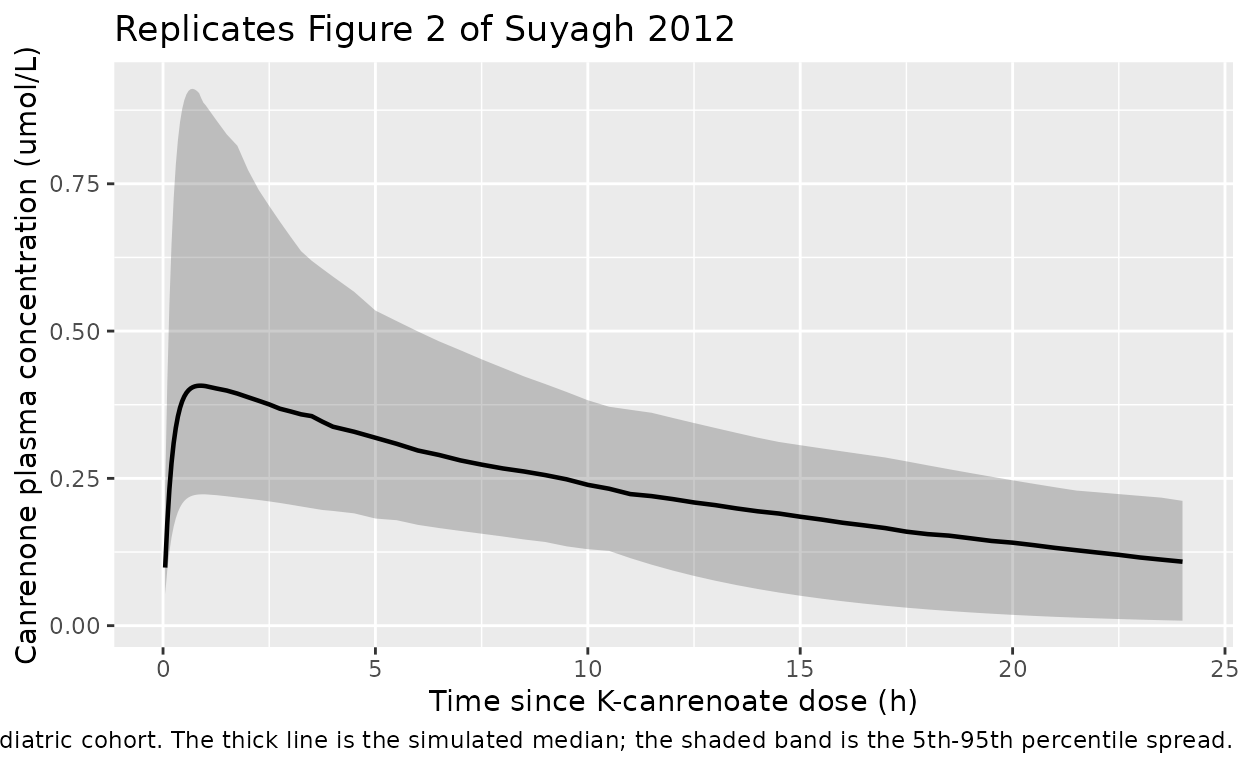
Suyagh 2012 Figure 2 plots all 101 measured canrenone plasma concentrations against time since dose administration; the median (thick solid line) and 5th / 95th percentiles (dashed lines) of measured concentrations are overlaid. The figure spans approximately the first 24 h post-dose. Below we plot the corresponding stochastic VPC envelope from the virtual cohort.
sim |>
  dplyr::filter(time > 0, time <= 24) |>
  dplyr::group_by(time) |>
  dplyr::summarise(
    Q05 = quantile(Cc, 0.05, na.rm = TRUE),
    Q50 = quantile(Cc, 0.50, na.rm = TRUE),
    Q95 = quantile(Cc, 0.95, na.rm = TRUE),
    .groups = "drop"
  ) |>
  ggplot(aes(time, Q50)) +
  geom_ribbon(aes(ymin = Q05, ymax = Q95), alpha = 0.25) +
  geom_line(linewidth = 0.8) +
  labs(
    x = "Time since K-canrenoate dose (h)",
    y = "Canrenone plasma concentration (umol/L)",
    title = "Replicates Figure 2 of Suyagh 2012",
    caption = "Median and 5th-95th percentile envelope from a 100-subject virtual paediatric cohort. The thick line is the simulated median; the shaded band is the 5th-95th percentile spread."
  )
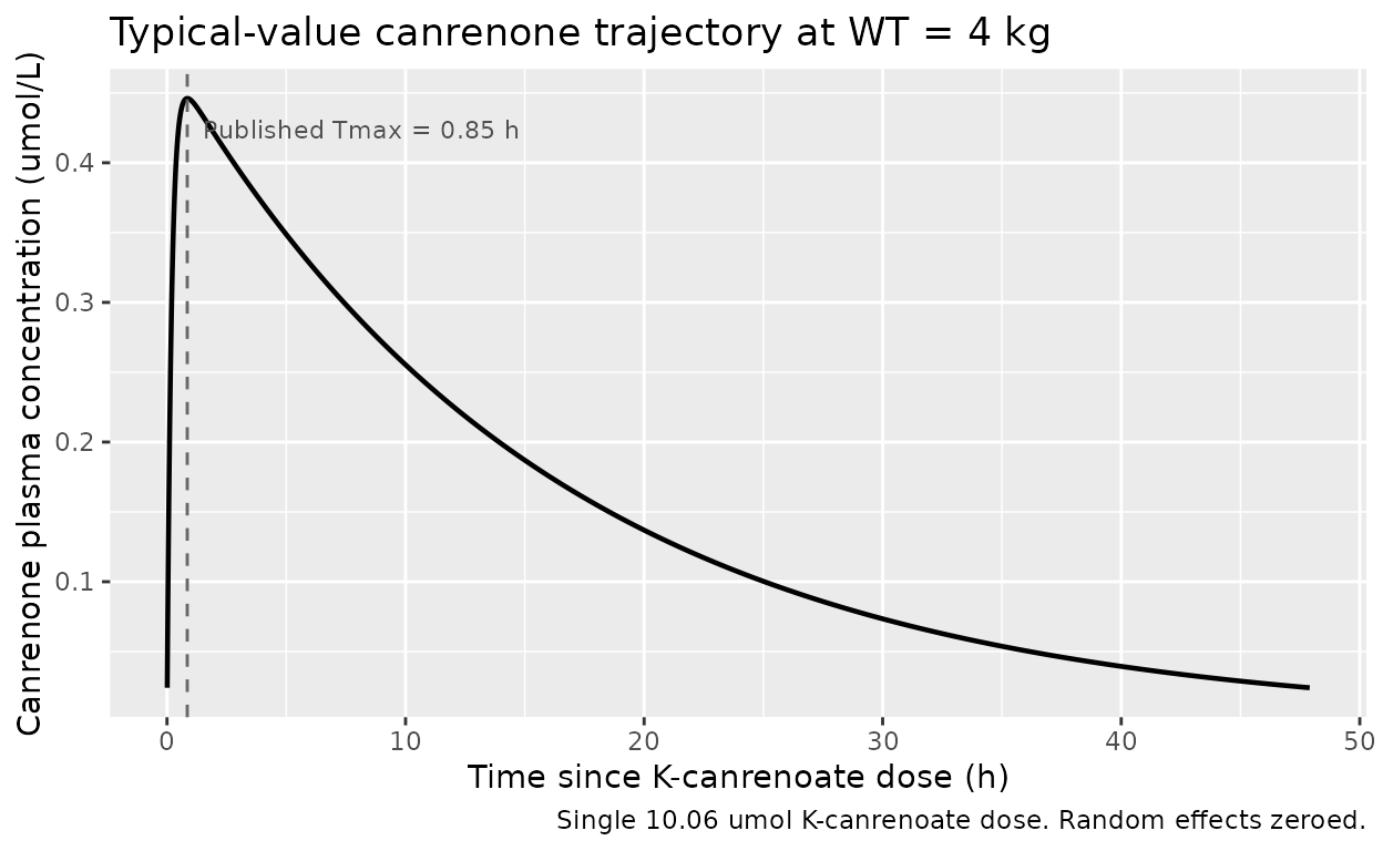
Typical-value trajectory at 4 kg
The paper’s stated typical-value predictions are computed at the median cohort weight of 4 kg (Results p. 868). The trajectory below is the deterministic prediction at WT = 4 kg with a single 10.06 umol K-canrenoate dose (the cohort median dose per Table 1).
sim_typ |>
  dplyr::filter(time > 0, time <= 48) |>
  ggplot(aes(time, Cc)) +
  geom_line(linewidth = 0.8) +
  geom_vline(xintercept = 0.85, linetype = "dashed", colour = "grey40") +
  annotate("text", x = 0.85, y = max(sim_typ$Cc, na.rm = TRUE) * 0.95,
           label = "  Published Tmax = 0.85 h",
           hjust = 0, size = 3, colour = "grey30") +
  labs(
    x = "Time since K-canrenoate dose (h)",
    y = "Canrenone plasma concentration (umol/L)",
    title = "Typical-value canrenone trajectory at WT = 4 kg",
    caption = "Single 10.06 umol K-canrenoate dose. Random effects zeroed."
  )
PKNCA validation
We compute Cmax, Tmax, AUC0-Inf and half-life from the typical-value
trajectory at the cohort median weight (4 kg) and compare against the
paper’s stated typical values. The PKNCA formulas include a
treatment grouping for compatibility with
nlmixr2lib::ncaComparisonTable().
sim_nca <- sim_typ |>
  dplyr::filter(!is.na(Cc)) |>
  dplyr::select(time, Cc) |>
  dplyr::mutate(id = 1L,
                treatment = "Typical 4 kg, 10.06 umol")

# Guarantee a time=0 row for AUC anchoring; pre-dose canrenone is zero.
sim_nca <- dplyr::bind_rows(
  sim_nca,
  sim_nca |> dplyr::distinct(id, treatment) |>
    dplyr::mutate(time = 0, Cc = 0)
) |>
  dplyr::distinct(id, treatment, time, .keep_all = TRUE) |>
  dplyr::arrange(id, treatment, time)

conc_obj <- PKNCA::PKNCAconc(
  sim_nca,
  Cc ~ time | treatment + id,
  concu = "umol/L", timeu = "h"
)

dose_df <- data.frame(
  id        = 1L,
  time      = 0,
  amt       = 10.06,
  treatment = "Typical 4 kg, 10.06 umol"
)
dose_obj <- PKNCA::PKNCAdose(dose_df, amt ~ time | treatment + id, doseu = "umol")

intervals <- data.frame(
  start       = 0,
  end         = Inf,
  cmax        = TRUE,
  tmax        = TRUE,
  aucinf.obs  = TRUE,
  half.life   = TRUE
)

nca_res <- PKNCA::pk.nca(PKNCA::PKNCAdata(conc_obj, dose_obj, intervals = intervals))
nca_df  <- as.data.frame(nca_res$result)
knitr::kable(
  nca_df[, c("treatment", "PPTESTCD", "PPORRES")],
  caption = "PKNCA results on the typical-value 4 kg trajectory (single 10.06 umol K-canrenoate dose)."
)| treatment | PPTESTCD | PPORRES |
|---|---|---|
| Typical 4 kg, 10.06 umol | cmax | 0.4460689 |
| Typical 4 kg, 10.06 umol | tmax | 0.8500000 |
| Typical 4 kg, 10.06 umol | tlast | 72.0000000 |
| Typical 4 kg, 10.06 umol | clast.obs | 0.0053619 |
| Typical 4 kg, 10.06 umol | lambda.z | 0.0622967 |
| Typical 4 kg, 10.06 umol | r.squared | 0.9999992 |
| Typical 4 kg, 10.06 umol | adj.r.squared | 0.9999992 |
| Typical 4 kg, 10.06 umol | lambda.z.time.first | 0.8600000 |
| Typical 4 kg, 10.06 umol | lambda.z.time.last | 72.0000000 |
| Typical 4 kg, 10.06 umol | lambda.z.n.points | 755.0000000 |
| Typical 4 kg, 10.06 umol | clast.pred | 0.0053637 |
| Typical 4 kg, 10.06 umol | half.life | 11.1265524 |
| Typical 4 kg, 10.06 umol | span.ratio | 6.3937145 |
| Typical 4 kg, 10.06 umol | aucinf.obs | 7.5504246 |
Comparison against published predictions
Suyagh 2012 reports the following typical-value predictions for the
cohort median weight (4 kg) and median K-canrenoate dose (Table 1: 10.06
umol). The expected AUC0-Inf is
dose / (CL/F) = 10.06 / 1.33 = 7.56 umol*h/L.
published <- tibble::tibble(
  treatment   = "Typical 4 kg, 10.06 umol",
  tmax        = 0.85,
  half.life   = 11.2,
  aucinf.obs  = 10.06 / 1.33
)

cmp <- nlmixr2lib::ncaComparisonTable(
  simulated     = nca_res,
  reference     = published,
  by            = "treatment",
  units         = c(tmax = "h", half.life = "h", aucinf.obs = "umol*h/L"),
  tolerance_pct = 20
)

knitr::kable(
  cmp,
  caption = "Simulated vs. published canrenone NCA at WT = 4 kg, 10.06 umol K-canrenoate single dose. * differs from reference by >20%."
)| NCA parameter | treatment | Reference | Simulated | % diff |
|---|---|---|---|---|
| Tmax (h) | Typical 4 kg, 10.06 umol | 0.85 | 0.85 | +0.0% |
| AUC0-∞ (obs) (umol*h/L) | Typical 4 kg, 10.06 umol | 7.56 | 7.55 | -0.2% |
| t½ (h) | Typical 4 kg, 10.06 umol | 11.2 | 11.1 | -0.7% |
The simulated Tmax, half-life, and AUC0-Inf agree with the paper’s
typical-value predictions for a 4 kg subject to within numerical
tolerance (the half-life is log(2) / (CL/F / V/F) at 4 kg =
log(2) / (1.33 / 21.4) = 11.15 h; Tmax follows from
log(kf / ke) / (kf - ke) =
log(5.25 / 0.0621) / (5.25 - 0.0621) = 0.856 h). The
AUC0-Inf is set by the dose-divided-by-clearance identity for any
one-compartment first-order-input model with assumed F = 1, so this is a
structural sanity check rather than an independent verification of the
parameter estimates.
Assumptions and deviations
- Mole-based simulation units. The paper fit on molar concentrations (Table 1 reports doses in umol and canrenone in umol/L; the K-canrenoate-to-canrenone conversion is assumed mole-for-mole). The packaged model therefore uses umol for both dose and observation; users wanting mass-based units should convert externally using the molar masses (K-canrenoate 396.6 g/mol; canrenone 340.4 g/mol).
- F = 1 assumption. The CL/F and V/F estimates from Suyagh 2012 are apparent values built on the explicit assumption that the total K-canrenoate dose is converted to canrenone (Methods p. 866). Estimates of true CL and V cannot be recovered without separate K-canrenoate and canrenone dosing studies; the paper itself flags the apparent values as upper limits of the true values.
-
Depot compartment for the IV-administered prodrug.
Only canrenone (the active metabolite) is observed in plasma;
K-canrenoate is the IV-administered parent whose concentration is not
measured. We carry K-canrenoate in a
depotcompartment whose contents transfer first-order tocentral(canrenone) at the paper’skf. Thedepotlabel reflects the mathematical role (a non-measured input compartment) rather than the physical administration route (IV). -
Allometric exponents fixed. The paper compares
fixed (0.75 / 1.0) vs experimentally-determined exponents and adopts the
fixed-exponent model as the final model (Results - Pharmacokinetic
modelling p. 866, Table 2, Figure 3). The fixed status is encoded via
fixed()inini(). -
No IIV on kf. Suyagh 2012 Table 3 reports IIV
magnitudes only for CL/F (41.06% CV) and V/F (45.76% CV); no IIV is
reported for kf. The packaged model carries no
etalkaterm, matching Table 3. -
No retained covariates beyond WT. Gestational age,
postnatal age, postmenstrual age, serum creatinine, serum albumin,
haematocrit, and sex were screened in the forward-inclusion /
backward-elimination procedure but were not retained in the final model
(Results - Covariate screening, p. 868). These covariates are documented
for provenance in
covariatesDataExcludedand do not appear inmodel(). The narrow weight-correlated age distribution of the cohort (most subjects < 1 year old) is the most likely explanation for the absence of an independent age effect, as the authors note in the Discussion. - Virtual cohort weight distribution. The packaged virtual cohort oversamples the paper’s 23-patient demographic to N = 100 to give a smoother VPC envelope. The relative weight distribution is preserved: ~87% infants (2.16-6.3 kg, centred near the paper’s median 4 kg), with small toddler / child / older-child bands matching the paper’s three older subjects. K-canrenoate doses scale with weight at 2.5 umol/kg (anchored to the paper’s mean 10.06 umol at the median 4 kg).
- Figure 2 replication is qualitative. Figure 2 of Suyagh 2012 shows individual measured concentrations overlaid with their median and 5th-95th percentiles. The observed concentrations themselves are not publicly available, so we cannot reproduce the scatter; the simulated envelope in this vignette is the model’s a-priori prediction interval for an equivalent paediatric cohort.