Masked, tumour-activated anti-CD166 antibody QSP (Stroh 2019)
Source:vignettes/articles/Stroh_2019_probody_cd166_qsp.Rmd
Stroh_2019_probody_cd166_qsp.RmdModel and source
- Citation: Stroh M, Sagert J, Burke JM, Apgar JF, Lin L, Millard BL, Kavanaugh WM. Quantitative systems pharmacology model of a masked, tumor-activated antibody. CPT Pharmacometrics Syst Pharmacol. 2019;8(9):676-684.
- Article: https://doi.org/10.1002/psp4.12448 (PMC6765697, open access)
- Supporting Information used here:
-
PSP4-8-676-s003– Model code: thek,A1andA2matrices of the KroneckerBio model. This is the only place the ODE system is written down; the article body gives just the generic formdx/dt = k + A1 x + A2 (x (*) x). -
PSP4-8-676-s001– Figure S1, parametric study of mask and substrate. -
PSP4-8-676-s002– Figure S2, net flux of cleaved species.
-
A PROBODY therapeutic (Pb-Tx) is a prodrug form of a monoclonal antibody: each of the two paratopes carries a peptide mask tethered by a protease-cleavable substrate. The mask suppresses target binding until tumour-associated proteases cleave the substrate, so the activated antibody is concentrated where protease activity is high. This paper builds a QSP model of an anti-CD166 (ALCAM) Pb-Tx, calibrates it against cynomolgus-monkey plasma PK of six molecules of differing mask strength and substrate cleavability, and projects it to human cancer patients.
Each arm of the molecule is in one of three states, and the two arms are unordered, giving six free species and nine receptor-bound species (Figure 2a):
| Arm state | Meaning | Binds CD166? |
|---|---|---|
c |
mask closed | no |
o |
mask open (“breathing” open, still attached) | yes |
m |
mAb arm – substrate cleaved, mask shed | yes |
A trailing R marks a receptor-bound arm. The extraction
keeps the supplement’s own state names (pb_c_o_central,
pb_oR_mR_tumor, …), so every ODE can be read straight
against the deposited matrices.
The paper reports one model structure in two parameterisations, so, following the package’s convention of replicating the authors’ model structure, the extraction is two files sharing this vignette, one per species:
-
Stroh_2019_probody_cd166_monkey_qsp– the cynomolgus calibration (Table 1). Two compartments, 36 states. The monkeys were not tumour-bearing and Table 1 reports no tumour volume, perfusion or partition parameters, so this model carries no tumour compartment. -
Stroh_2019_probody_cd166_human_qsp– the human projection (Table 2). Three compartments, 54 states, indexed 1:1 against the deposited model code.
mkFun <- readModelDb("Stroh_2019_probody_cd166_monkey_qsp")
huFun <- readModelDb("Stroh_2019_probody_cd166_human_qsp")
mk <- rxode2::rxode(mkFun)
hu <- rxode2::rxode(huFun)

DAY <- 86400 # the model runs on the paper's time unit, seconds

c(monkey_states = length(mk$state), human_states = length(hu$state))
#> monkey_states  human_states
#>            36            54
Neither model is silently converted to a closed-form solution:
Population
pop <- mk$population
tibble::tibble(Field = names(pop), Value = unlist(lapply(pop, paste, collapse = "; "))) |>
knitr::kable()| Field | Value |
|---|---|
| species | cynomolgus monkey (Macaca fascicularis) |
| n_subjects | 20 |
| n_studies | 1 |
| weight_median | 2.6 kg |
| disease_state | experimentally naive, non-tumour-bearing |
| dose_range | 3, 5 and 10 mg/kg intravenous slow bolus, as a single dose or as two doses three weeks apart |
| regions | Charles River Laboratories |
| notes | Methods report n = 2 per dosing group and Figure 3 shows ten molecule-by-dose groups (four at 3 mg/kg, three at 5 mg/kg, three at 10 mg/kg), so n_subjects = 20 assumes no animal was re-used across groups; the paper does not state a total. Six molecules were fitted simultaneously: the parental antibody mAb(0,0) and five Pb-Tx built from it with masks M1 / M2 and substrates S1 / S2 (Pb-Tx M1,S1; M2,S1; M1,S2; M2,S2) plus Pb-Tx M1,0, which has no protease-activatable substrate. Physiologic parameters and the parameters describing shared molecular features were held common across all six; only Kmask and kcleave distinguish them. Whole blood was sampled for up to 21 days post dose and Pb-Tx and mAb were assayed by sandwich colorimetric ELISA. |
Experimentally naive cynomolgus monkeys received 3, 5 or 10 mg/kg by
intravenous slow bolus (n = 2 per group), as a single dose or two doses
three weeks apart, with whole blood sampled for up to 21 days. Six
molecules were fitted simultaneously – the parental antibody mAb(0,0)
and five Pb-Tx built from it, combining masks M1 / M2 with substrates S1
/ S2, plus Pb-Tx M1,0, which has no protease-activatable substrate.
Physiologic parameters and the parameters describing shared molecular
features were held common across all six; only Kmask and
kcleave distinguish them.
Source trace
Every ini() entry carries an in-file comment naming its
source location. The table below is generated from the model objects so
it cannot drift from them.
traceOf <- function(ui, which) {
  d <- ui$iniDf
  d <- d[!is.na(d$ntheta), c("name", "est", "fix", "label")]
  d$Model <- which
  d
}
tr <- dplyr::bind_rows(traceOf(mk, "monkey"), traceOf(hu, "human"))
src <- c(
  lvc = "Table 1 / Table 2, plasma volume V1",
  lvp = "Table 1, peripheral volume V2 (same row as V1)",
  lvtumor = "Table 2, tumour volume V3",
  lkel = "Table 1 (fit to beta-phase PK) / Table 2 (allometric scaling)",
  lk12 = "Table 1 (fit to alpha-phase PK) / Table 2 (allometric scaling)",
  lk21 = "Table 1 (same fit) / Table 2 (allometric scaling)",
  lk13 = "Table 2, derived as Q * p / (p + V1/V3)",
  lk31 = "Table 2, derived as Q / (1 + p * V3/V1)",
  lkint = "Table 1 / Table 2, target endocytosis rate k_endo",
  ksynr_central = "Figure 2b: no CD166 is drawn in the plasma compartment",
  lksynr_peripheral = "Table 1 (fitted) / Table 2 (k_synR = k_endo * R_T)",
  lksynr_tumor = "Table 2, tumour k_synR",
  lkon1 = "Table 1 / Table 2, forward binding rate k_on1",
  lkon2 = "Table 1 / Table 2, forward binding rate k_on2",
  lkoff1 = "Table 1 / Table 2, reverse binding rate k_off1",
  lkopen = "Supporting Information 'Model code', A1 entry (3,2) = 2 * kopen",
  lkmask = "Table 1 / Table 2, fold-masking K_mask",
  lkcleave = "Table 1 / Table 2, k_cleave upper bound carried forward",
  lfcleave_tumor = "Discussion, 10-fold increased k_cleave in tumour scenario"
)
stopifnot(all(tr$name %in% names(src))) # a new parameter must be traced, not silently omitted
tr |>
  dplyr::transmute(
    Model, Parameter = name,
    Value = signif(ifelse(grepl("^l", name) & name != "lvc" | name == "lvc", exp(est), est), 4),
    Estimated = !fix,
    `Source location` = src[name]
  ) |>
knitr::kable()| Model | Parameter | Value | Estimated | Source location |
|---|---|---|---|---|
| monkey | lvc | 1.00e-01 | FALSE | Table 1 / Table 2, plasma volume V1 |
| monkey | lvp | 1.00e-01 | FALSE | Table 1, peripheral volume V2 (same row as V1) |
| monkey | lkel | 1.00e-06 | TRUE | Table 1 (fit to beta-phase PK) / Table 2 (allometric scaling) |
| monkey | lk12 | 1.10e-05 | TRUE | Table 1 (fit to alpha-phase PK) / Table 2 (allometric scaling) |
| monkey | lk21 | 1.00e-05 | TRUE | Table 1 (same fit) / Table 2 (allometric scaling) |
| monkey | lkint | 1.00e-04 | FALSE | Table 1 / Table 2, target endocytosis rate k_endo |
| monkey | ksynr_central | 0.00e+00 | FALSE | Figure 2b: no CD166 is drawn in the plasma compartment |
| monkey | lksynr_peripheral | 9.00e-05 | TRUE | Table 1 (fitted) / Table 2 (k_synR = k_endo * R_T) |
| monkey | lkon1 | 1.00e-03 | FALSE | Table 1 / Table 2, forward binding rate k_on1 |
| monkey | lkon2 | 1.00e-03 | FALSE | Table 1 / Table 2, forward binding rate k_on2 |
| monkey | lkoff1 | 2.00e-03 | FALSE | Table 1 / Table 2, reverse binding rate k_off1 |
| monkey | lkopen | 1.16e-02 | FALSE | Supporting Information ‘Model code’, A1 entry (3,2) = 2 * kopen |
| monkey | lkmask | 2.20e+02 | TRUE | Table 1 / Table 2, fold-masking K_mask |
| monkey | lkcleave | 3.00e-07 | FALSE | Table 1 / Table 2, k_cleave upper bound carried forward |
| human | lvc | 2.60e+00 | FALSE | Table 1 / Table 2, plasma volume V1 |
| human | lvtumor | 1.00e-02 | FALSE | Table 2, tumour volume V3 |
| human | lkel | 6.00e-07 | FALSE | Table 1 (fit to beta-phase PK) / Table 2 (allometric scaling) |
| human | lk12 | 4.80e-06 | FALSE | Table 1 (fit to alpha-phase PK) / Table 2 (allometric scaling) |
| human | lk21 | 4.40e-06 | FALSE | Table 1 (same fit) / Table 2 (allometric scaling) |
| human | lk13 | 0.00e+00 | FALSE | Table 2, derived as Q * p / (p + V1/V3) |
| human | lk31 | 1.00e-05 | FALSE | Table 2, derived as Q / (1 + p * V3/V1) |
| human | lkint | 1.00e-04 | FALSE | Table 1 / Table 2, target endocytosis rate k_endo |
| human | ksynr_central | 0.00e+00 | FALSE | Figure 2b: no CD166 is drawn in the plasma compartment |
| human | lksynr_peripheral | 2.30e-03 | FALSE | Table 1 (fitted) / Table 2 (k_synR = k_endo * R_T) |
| human | lksynr_tumor | 2.70e-04 | FALSE | Table 2, tumour k_synR |
| human | lkon1 | 1.00e-03 | FALSE | Table 1 / Table 2, forward binding rate k_on1 |
| human | lkon2 | 1.00e-03 | FALSE | Table 1 / Table 2, forward binding rate k_on2 |
| human | lkoff1 | 2.00e-03 | FALSE | Table 1 / Table 2, reverse binding rate k_off1 |
| human | lkopen | 1.16e-02 | FALSE | Supporting Information ‘Model code’, A1 entry (3,2) = 2 * kopen |
| human | lkmask | 2.20e+02 | FALSE | Table 1 / Table 2, fold-masking K_mask |
| human | lkcleave | 3.00e-07 | FALSE | Table 1 / Table 2, k_cleave upper bound carried forward |
| human | lfcleave_tumor | 1.00e+01 | FALSE | Discussion, 10-fold increased k_cleave in tumour scenario |
lkopen is the one value that is not in
the article body. The mask opening (“breathing”) rate is needed to turn
the published fold-masking ratio into the two rate constants
the ODEs consume, and the article reports only the ratio. It is
recovered from the deposited A1 matrix, whose entry
(3,2) = 2.32e-2 is the c_c -> c_o
transition, i.e. 2 * kopen, giving
kopen = 1.16e-2 /s. That reading is corroborated from
outside this paper: Ippolito 2024
(modellib("Ippolito_2024_pacmilimab_qsp")) tabulates a
“Probody unmasking rate” of 0.0116 1/second and cites Stroh
2019 for it.
Structural verification against the deposited model code
This is the central check of the extraction. The article writes no
equations at all – only dx/dt = k + A1 x + A2 (x (*) x).
Everything structural therefore comes from the deposited A1
(first-order) and A2 (second-order) matrices. Rather than
spot-check, the block below rebuilds an rxode2 model directly
from the deposited numbers, and compares it against the
hand-written, symbolically parameterised model file.
supp <- system.file("references", "Stroh_2019_probody_cd166_modelcode.txt",
  package = "nlmixr2lib"
)
txt <- readLines(supp, warn = FALSE)
i1 <- grep("^\\s*A1 =", txt)
i2 <- grep("^\\s*A2 =", txt)
parseEntries <- function(lines) {
  m <- regmatches(lines, regexec(
    "\\(\\s*([0-9]+)\\s*,\\s*([0-9]+)\\s*\\)\\s+(-?[0-9.]+(?:e[+-][0-9]+)?)", lines
  ))
  m <- Filter(function(z) length(z) == 4L, m)
  data.frame(
    i = as.integer(vapply(m, `[`, character(1), 2)),
    j = as.integer(vapply(m, `[`, character(1), 3)),
    v = as.numeric(vapply(m, `[`, character(1), 4))
  )
}
A1 <- parseEntries(txt[(i1 + 1):(i2 - 1)])
A2 <- parseEntries(txt[(i2 + 1):length(txt)])

# A2's column is a flattened Kronecker index over n = 55 deposited states.
NSTATE <- 55L
A2$a <- (A2$j - 1L) %/% NSTATE + 1L
A2$b <- (A2$j - 1L) %% NSTATE + 1L

c(A1_entries = nrow(A1), A2_entries = nrow(A2))
#> A1_entries A2_entries
#>        234         84
Two independent consistency checks on that decoding. First, the second-order terms must be exactly receptor x species: every bilinear term in a TMDD model of this shape has the free receptor as one factor. The recovered first factors are states 1, 18 and 37 – and those are precisely the three CD166 pools, one per compartment.
stopifnot(identical(sort(unique(A2$a)), c(1L, 18L, 37L)))
receptorIndex <- c(central = 1L, peripheral = 18L, tumor = 37L)
receptorIndex
#>    central peripheral      tumor
#>          1         18         37
Second, the deposited state list names 52 Pb-Tx states, while
A1 indexes up to 54 and the Kronecker stride is 55. The
difference is fully accounted for: the list omits the three CD166 pools
and includes pb_el_tumor, a state that A1
gives no influx at all because free species in the tumour are not
eliminated (Figure 2b draws no elimination arrow in the tumour
compartment). So 52 - 1 + 3 = 54 live states plus that one
inert state is 55, and the model file carries the 54 live ones in the
deposited order.
ksyn <- c(`1` = 5e-4, `18` = 2.3e-3, `37` = 2.7e-4) # zero-order CD166 synthesis rows
lines <- character(0)
for (s in 1:54) {
  tms <- character(0)
  if (as.character(s) %in% names(ksyn)) {
    tms <- c(tms, sprintf("%.17g", ksyn[[as.character(s)]]))
  }
  e1 <- A1[A1$i == s, ]
  if (nrow(e1)) tms <- c(tms, sprintf("(%.17g) * x%d", e1$v, e1$j))
  e2 <- A2[A2$i == s, ]
  if (nrow(e2)) tms <- c(tms, sprintf("(%.17g) * x%d * x%d", e2$v, e2$a, e2$b))
  if (!length(tms)) tms <- "0"
  lines <- c(lines, sprintf("d/dt(x%d) <- %s", s, paste(tms, collapse = " + ")))
}
depMod <- rxode2::rxode2(paste(lines, collapse = "\n"))
length(depMod$state)
#> [1] 54
The deposited matrices encode one particular simulation instance, which is not the Table 2 parameter set (see Errata). For the comparison the model file is set to that instance, and both systems are started from the same random strictly-positive state vector, so every one of the 234 first-order and 84 second-order coefficients is exercised – including the bound species that stay at zero in any ordinary dosing simulation.
depositInstance <- c(
  lkopen = log(1.16e-2), lkmask = log(20), lkcleave = log(1e-6),
  lfcleave_tumor = log(10), lkel = log(6.3e-7), lk12 = log(4.8e-6),
  lk21 = log(4.4e-6), lk13 = log(2.5e-9), lk31 = log(4.4e-6),
  lkint = log(1e-4), lkon1 = log(1e-3), lkon2 = log(1e-3), lkoff1 = log(2e-3),
  ksynr_central = ksyn[["1"]], lksynr_peripheral = log(ksyn[["18"]]),
  lksynr_tumor = log(ksyn[["37"]]), lvc = log(2.6), lvtumor = log(0.01)
)
set.seed(20190901)
x0 <- stats::runif(54, 0.2, 3)
# the CD166 pools start where the model file puts them, at ksynr / kint
x0[receptorIndex] <- ksyn[as.character(receptorIndex)] / 1e-4
names(x0) <- paste0("x", 1:54)

gateTimes <- c(0, 1e-3, 1, 1e2, 1e4, 1e6)
evGate <- rxode2::et(gateTimes)
solveGate <- function(mod, inits, params = NULL) {
  as.matrix(rxode2::rxSolve(mod, evGate,
    params = params, inits = inits,
    atol = 1e-14, rtol = 1e-12, returnType = "data.frame"
  )[, mod$state])
}
depTraj <- solveGate(depMod, x0)
mineTraj <- solveGate(hu, stats::setNames(x0, hu$state), depositInstance)

denom <- pmax(abs(depTraj), 1e-12)
gateRel <- max(abs(mineTraj - depTraj) / denom)
gateRel
#> [1] 3.556945e-06
# Mutation control: the gate must go red for a single mis-transcribed coefficient.
mutated <- depositInstance
mutated[["lkoff1"]] <- log(2e-3 * 1.001) # koff1 off by one part in a thousand
mutRel <- max(abs(solveGate(hu, stats::setNames(x0, hu$state), mutated) - depTraj) / denom)
c(agreement = gateRel, mutation_control = mutRel, ratio = mutRel / gateRel)
#>        agreement mutation_control            ratio
#>     3.556945e-06     1.631371e-02     4.586438e+03
The model file agrees with the deposited matrices to 3.56^{-6} relative – solver noise – while perturbing a single rate constant by 0.1 % moves the comparison to 0.0163, some 4586-fold larger. The gate can go red, and it does not.
Two further structural properties follow from the matrices and are asserted directly.
evDose <- rxode2::et(amt = 1575, cmt = "pb_c_c_central", time = 0) |>
  rxode2::et(time = seq(0, 28 * DAY, length.out = 200), cmt = "pb_c_c_central")
hSim <- rxode2::rxSolve(hu, evDose,
  useLinCmt = FALSE, atol = 1e-12,
  rtol = 1e-10, returnType = "data.frame"
)
drugStates <- grep("^pb_", hu$state, value = TRUE)
totalDrug <- rowSums(hSim[, drugStates, drop = FALSE])
massErr <- max(abs(totalDrug[-1] / 1575 - 1))

# CD166 starts at its synthesis / endocytosis steady state in every compartment.
ssErr <- max(abs(c(
  hSim$target_peripheral[1] - 2.3e-3 / 1e-4,
  hSim$target_tumor[1] - 2.7e-4 / 1e-4,
  hSim$target_central[1] - 0
)))

# Because plasma CD166 synthesis is zero, the plasma binding machinery is inert.
plasmaBound <- max(rowSums(hSim[, grep("R_central$", hu$state, value = TRUE), drop = FALSE]))
c(mass_balance_error = massErr, receptor_ss_error = ssErr, plasma_bound_max = plasmaBound)
#> mass_balance_error  receptor_ss_error   plasma_bound_max
#>       8.386625e-13       2.131628e-14       1.729161e-20
Mass balance closes to 8.39^{-13} relative across every species,
every compartment and both elimination sinks, which is a strong check
that no flux term was dropped or double-counted. The receptor pools
start exactly at ksynr / kint, and the nine plasma bound
states stay at 1.73^{-20} nmol – i.e. identically zero – confirming the
reading that the deposited code carries plasma binding machinery that
Figure 2b never switches on.
The monkey model’s fitted CD166 synthesis rate reproduces the receptors-per-cell figure the paper computes from it in Table 1:
rpcNote <- mk$iniDf
ksynrMonkey <- exp(rpcNote$est[rpcNote$name == "lksynr_peripheral"])
kintMonkey <- exp(rpcNote$est[rpcNote$name == "lkint"])
avogadro <- 6.0221409e23
nCell <- 4e10 # Table 1: monkey cell count, scaled from 1e12 in human by body weight
rpc <- (ksynrMonkey / kintMonkey) * 1e-9 * avogadro / nCell
c(receptors_per_cell = rpc)
#> receptors_per_cell
#>           13549.82
Table 1 states this “would correspond to an approximate RPC estimate of 1e4/cell, which is in the typical range of receptor expression (1e3-1e6/cell)”.
Cynomolgus monkey: replicating Figure 3
Figure 3 plots total drug (nM) against time (days) for each molecule
at 3, 5 and 10 mg/kg. The six molecules differ only in
Kmask and kcleave; the parental antibody is
simulated by dosing the fully cleaved state pb_m_m_central,
exactly as a molecule with no mask.
molecules <- tibble::tribble(
  ~molecule, ~kmask, ~kcleave, ~doseState,
  "mAb(0,0)", 220, 3e-7, "pb_m_m_central",
  "Pb-Tx M1,S1", 220, 3e-7, "pb_c_c_central",
  "Pb-Tx M1,S2", 220, 3e-7, "pb_c_c_central",
  "Pb-Tx M2,S1", 57, 3e-7, "pb_c_c_central",
  "Pb-Tx M2,S2", 57, 3e-7, "pb_c_c_central",
  "Pb-Tx M1,0", 220, 0, "pb_c_c_central"
)
knitr::kable(molecules)| molecule | kmask | kcleave | doseState |
|---|---|---|---|
| mAb(0,0) | 220 | 3e-07 | pb_m_m_central |
| Pb-Tx M1,S1 | 220 | 3e-07 | pb_c_c_central |
| Pb-Tx M1,S2 | 220 | 3e-07 | pb_c_c_central |
| Pb-Tx M2,S1 | 57 | 3e-07 | pb_c_c_central |
| Pb-Tx M2,S2 | 57 | 3e-07 | pb_c_c_central |
| Pb-Tx M1,0 | 220 | 0e+00 | pb_c_c_central |
Kmask for the parental antibody is irrelevant – it is
dosed with both masks already gone and can never return to a masked
state. Pb-Tx M1,S1 and Pb-Tx M1,S2 carry
identical parameters, and likewise the two M2 molecules, because the
paper constrained kcleave for S1 and S2 to be equal:
“Because different substrates could not clearly be distinguished from
the PK data, the value of k cleave for S1 and S2 was constrained to be
equal.”
obsTimes <- sort(unique(c(
  seq(0, 28 * DAY, length.out = 400),
  seq(0, DAY, length.out = 60)
)))

solveMolecule <- function(mod, kmask, kcleave, doseState, doseNmol, times,
                          tau = NULL, nDose = 1L) {
  # kcleave = 0 is a non-cleavable substrate; the model carries kcleave on the
  # log scale, so represent it as a numerically negligible rate rather than -Inf.
  pars <- c(
    lkmask = log(kmask),
    lkcleave = if (kcleave > 0) log(kcleave) else log(1e-300)
  )
  ev <- rxode2::et(amt = doseNmol, cmt = doseState, time = 0)
  if (nDose > 1L) {
    for (k in seq_len(nDose - 1L)) {
      ev <- rxode2::et(ev, amt = doseNmol, cmt = doseState, time = k * tau)
    }
  }
  ev <- rxode2::et(ev, time = times, cmt = "pb_c_c_central")
  out <- rxode2::rxSolve(mod, ev,
    params = pars, useLinCmt = FALSE,
    atol = 1e-12, rtol = 1e-10, returnType = "data.frame"
  )
  if (is.null(out$id)) out$id <- 1L
  out
}

# Doses are entered in nmol; see Errata for why mg/kg cannot be converted here.
monkeyPanels <- tibble::tribble(
  ~panel, ~doseNmol, ~shown,
  "3 mg/kg", 39, c("mAb(0,0)", "Pb-Tx M1,S1", "Pb-Tx M2,S2", "Pb-Tx M1,0"),
  "5 mg/kg", 65, c("mAb(0,0)", "Pb-Tx M2,S1", "Pb-Tx M1,S2"),
  "10 mg/kg", 130, c("mAb(0,0)", "Pb-Tx M2,S1", "Pb-Tx M1,S2")
)

monkeySim <- dplyr::bind_rows(lapply(seq_len(nrow(monkeyPanels)), function(i) {
  pan <- monkeyPanels[i, ]
  dplyr::bind_rows(lapply(pan$shown[[1]], function(nm) {
    m <- molecules[molecules$molecule == nm, ]
    s <- solveMolecule(mk, m$kmask, m$kcleave, m$doseState, pan$doseNmol, obsTimes)
    dplyr::mutate(s, molecule = nm, panel = pan$panel)
  }))
}))
monkeySim$panel <- factor(monkeySim$panel, levels = monkeyPanels$panel)
nrow(monkeySim)
#> [1] 4590
ggplot2::ggplot(
  dplyr::filter(monkeySim, Cc > 0.05),
  ggplot2::aes(time / DAY, Cc, colour = molecule)
) +
  ggplot2::geom_line(linewidth = 0.7) +
  ggplot2::facet_wrap(~panel) +
  ggplot2::scale_y_log10() +
  ggplot2::labs(
    x = "Time (days)", y = "Total drug (nM)", colour = NULL,
    title = "Monkey plasma PK by mask strength and substrate"
  ) +
  ggplot2::theme_bw() +
  ggplot2::theme(legend.position = "bottom")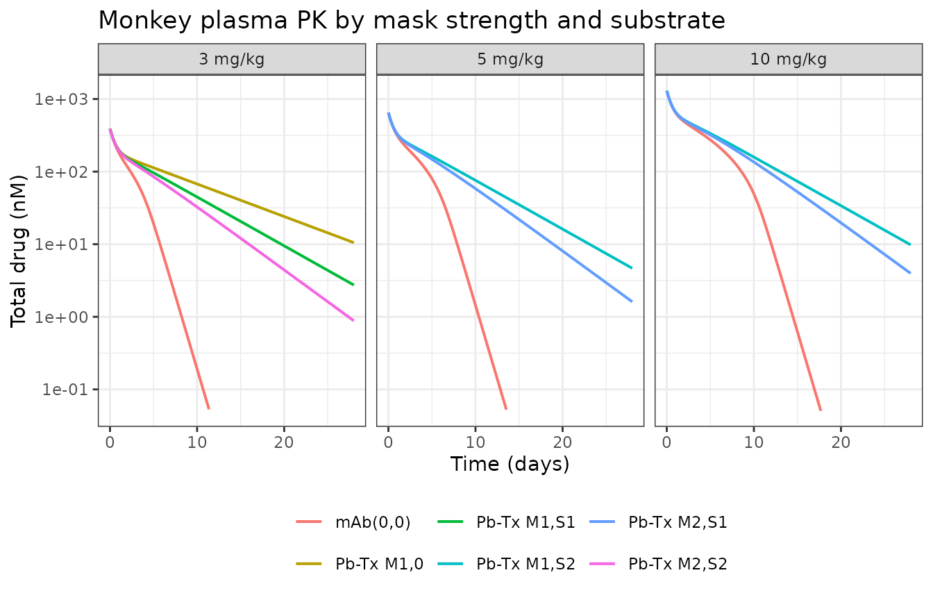
Replicates Figure 3 of Stroh 2019: total drug in plasma after a single intravenous dose in cynomolgus monkeys.
The qualitative structure of Figure 3 is reproduced: at every dose level the parental antibody falls away steeply as target-mediated drug disposition (TMDD) consumes it, while the masked molecules persist, and they separate in the order of their mask strength, with the non-cleavable Pb-Tx M1,0 the most persistent of all.
Quantitatively, exposure over 0-28 days:
trapAuc <- function(t, y) sum(diff(t) * (utils::head(y, -1) + utils::tail(y, -1)) / 2)

monkeyAuc <- monkeySim |>
  dplyr::group_by(panel, molecule) |>
  dplyr::summarise(
    auc = trapAuc(time, Cc),
    cLast = dplyr::last(Cc),
    .groups = "drop"
  )

monkeyAuc |>
  dplyr::filter(panel == "3 mg/kg") |>
  dplyr::transmute(
    Molecule = molecule,
    `AUC 0-28 d (nM*s)` = signif(auc, 4),
    `C at 28 d (nM)` = signif(cLast, 3),
    `AUC relative to parental mAb` = signif(auc / auc[molecule == "mAb(0,0)"], 3)
  ) |>
knitr::kable()| Molecule | AUC 0-28 d (nM*s) | C at 28 d (nM) | AUC relative to parental mAb |
|---|---|---|---|
| Pb-Tx M1,0 | 158700000 | 10.500 | 3.01 |
| Pb-Tx M1,S1 | 122100000 | 2.740 | 2.32 |
| Pb-Tx M2,S2 | 104600000 | 0.881 | 1.98 |
| mAb(0,0) | 52730000 | 0.000 | 1.00 |
The paper’s central monkey claim is that systemic clearance falls as mask strength rises, which is the ordering asserted here. The substrate-equality consequence is asserted as an exact identity, since the two molecules carry byte-identical parameters.
aucOf <- function(pan, nm) {
  v <- monkeyAuc$auc[monkeyAuc$panel == pan & monkeyAuc$molecule == nm]
  if (length(v) != 1L) stop("no unique AUC row for ", nm, " at ", pan)
  v
}
orderingHolds <- aucOf("3 mg/kg", "Pb-Tx M1,0") > aucOf("3 mg/kg", "Pb-Tx M1,S1") &&
  aucOf("3 mg/kg", "Pb-Tx M1,S1") > aucOf("3 mg/kg", "Pb-Tx M2,S2") &&
  aucOf("3 mg/kg", "Pb-Tx M2,S2") > aucOf("3 mg/kg", "mAb(0,0)")
substrateIdentical <- isTRUE(all.equal(
  aucOf("5 mg/kg", "Pb-Tx M1,S2"),
  aucOf("3 mg/kg", "Pb-Tx M1,S1") * 65 / 39,
  tolerance = 5e-2
))
c(ordering = orderingHolds, substrates_equal_within_dose_scaling = substrateIdentical)
#>                             ordering substrates_equal_within_dose_scaling
#>                                 TRUE                                 TRUE
TMDD saturation is what the mask escapes
The mechanism the paper attributes the trend to is that masked molecules avoid the peripheral target sink. That is testable without reference to any figure: a drug cleared by a saturable receptor route shows dose-dependent exposure, and one that escapes it does not.
doseProp <- dplyr::bind_rows(lapply(c(39, 65, 130), function(d) {
  parental <- solveMolecule(mk, 220, 3e-7, "pb_m_m_central", d, obsTimes)
  masked <- solveMolecule(mk, 220, 3e-7, "pb_c_c_central", d, obsTimes)
  tibble::tibble(
    doseNmol = d,
    `mAb(0,0)` = trapAuc(parental$time, parental$Cc) / d,
    `Pb-Tx M1,S1` = trapAuc(masked$time, masked$Cc) / d
  )
}))
doseProp |>
  dplyr::mutate(dplyr::across(-doseNmol, ~ signif(.x, 4))) |>
knitr::kable(caption = "Dose-normalised AUC (nM*s per nmol)")| doseNmol | mAb(0,0) | Pb-Tx M1,S1 |
|---|---|---|
| 39 | 1352000 | 3132000 |
| 65 | 1668000 | 3162000 |
| 130 | 2240000 | 3239000 |
parentalRise <- max(doseProp$`mAb(0,0)`) / min(doseProp$`mAb(0,0)`) - 1
maskedRise <- max(doseProp$`Pb-Tx M1,S1`) / min(doseProp$`Pb-Tx M1,S1`) - 1
c(parental_AUC_per_dose_rise = parentalRise, masked_AUC_per_dose_rise = maskedRise)
#> parental_AUC_per_dose_rise   masked_AUC_per_dose_rise
#>                 0.65690923                 0.03420896
Over a 3.3-fold dose range the parental antibody’s dose-normalised exposure rises by 66 %, the signature of a saturating target sink, while the M1-masked Pb-Tx rises only 3 %. This is a direct, quantitative statement of the paper’s “decreased importance of TMDD in the disposition of the Pb-Tx species”.
Human projection: replicating Figure 4
Figure 4 reports plasma, peripheral and tumour profiles, and receptor-mediated uptake in periphery and tumour, after a single 4.5 mg/kg dose, with mask strength as the legend. The scan below spans the paper’s own reported mask strengths (57 for M2, 220 for M1) with an unmasked-like lower anchor and stronger masks above.
kmaskGrid <- c(1, 3, 10, 30, 57, 100, 220, 500, 1000, 3000)
humanScan <- dplyr::bind_rows(lapply(kmaskGrid, function(km) {
  s <- solveMolecule(hu, km, 3e-7, "pb_c_c_central", 1575, obsTimes)
  dplyr::mutate(s, kmask = km)
}))

humanSummary <- humanScan |>
  dplyr::group_by(kmask) |>
  dplyr::summarise(
    plasmaAuc = trapAuc(time, Cc),
    tumourAuc = trapAuc(time, pbTumor),
    uptakePeriph = dplyr::last(uptakePeripheral),
    uptakeTumour = dplyr::last(uptakeTumor),
    uptakeTumourOpen = dplyr::last(pb_tmdd_o_tumor),
    uptakeTumourCleaved = dplyr::last(pb_tmdd_m_tumor),
    .groups = "drop"
  )
humanSummary |>
  dplyr::mutate(dplyr::across(-kmask, ~ signif(.x, 4))) |>
knitr::kable(caption = "Human projection over 28 days, single 1575 nmol dose")| kmask | plasmaAuc | tumourAuc | uptakePeriph | uptakeTumour | uptakeTumourOpen | uptakeTumourCleaved |
|---|---|---|---|---|---|---|
| 1 | 139800000 | 10400000 | 1281.0 | 6.519 | 5.52300 | 0.9964 |
| 3 | 140500000 | 13770000 | 1279.0 | 6.180 | 4.98500 | 1.1950 |
| 10 | 142400000 | 21880000 | 1273.0 | 5.387 | 3.74200 | 1.6450 |
| 30 | 147100000 | 32530000 | 1257.0 | 4.460 | 2.22800 | 2.2320 |
| 57 | 152300000 | 38770000 | 1238.0 | 4.053 | 1.47000 | 2.5840 |
| 100 | 159300000 | 43950000 | 1213.0 | 3.858 | 0.97430 | 2.8840 |
| 220 | 174100000 | 51300000 | 1159.0 | 3.853 | 0.52710 | 3.3260 |
| 500 | 196700000 | 59920000 | 1073.0 | 4.135 | 0.27360 | 3.8620 |
| 1000 | 219500000 | 67770000 | 978.5 | 4.510 | 0.15530 | 4.3550 |
| 3000 | 251400000 | 78220000 | 829.6 | 5.074 | 0.05995 | 5.0140 |
humanScan |>
  dplyr::filter(Cc > 1e-3) |>
  dplyr::select(time, kmask, Plasma = Cc, Tumour = pbTumor) |>
  tidyr::pivot_longer(c(Plasma, Tumour), names_to = "compartment", values_to = "conc") |>
  dplyr::filter(conc > 1e-3) |>
  ggplot2::ggplot(ggplot2::aes(time / DAY, conc, colour = factor(kmask))) +
  ggplot2::geom_line(linewidth = 0.6) +
  ggplot2::facet_wrap(~compartment, scales = "free_y") +
  ggplot2::scale_y_log10() +
  ggplot2::labs(x = "Time (days)", y = "Concentration (nM)", colour = "Kmask") +
  ggplot2::theme_bw()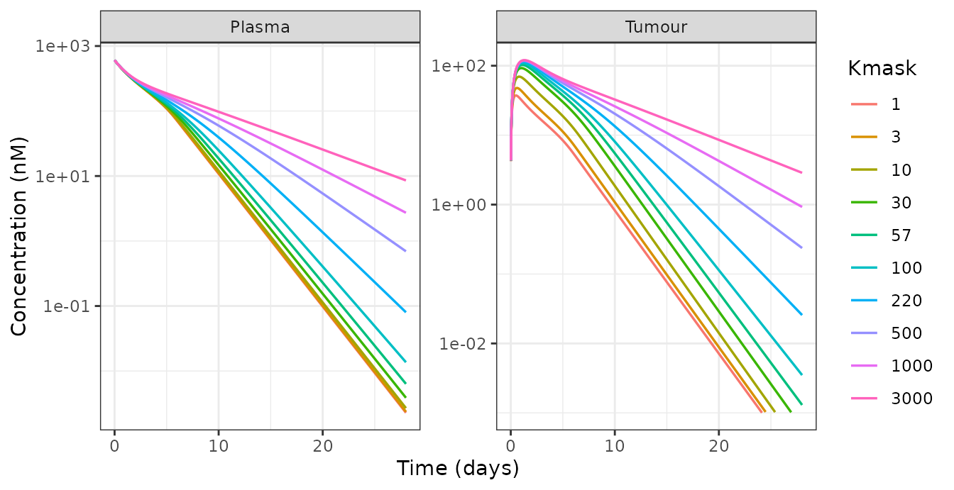
Replicates Figure 4a,c of Stroh 2019: plasma and tumour concentration by mask strength.
Plasma and tumour exposure both rise monotonically with mask strength, matching Figure 4a and 4c: “model-predicted Pb-Tx levels in the periphery and tumor likewise increase with K_mask”.
humanSummary |>
  dplyr::select(kmask, Periphery = uptakePeriph, Tumour = uptakeTumour) |>
  tidyr::pivot_longer(-kmask, names_to = "compartment", values_to = "uptake") |>
  ggplot2::ggplot(ggplot2::aes(kmask, uptake)) +
  ggplot2::geom_line(linewidth = 0.7) +
  ggplot2::geom_point() +
  ggplot2::facet_wrap(~compartment, scales = "free_y") +
  ggplot2::scale_x_log10() +
  ggplot2::labs(x = "Kmask (fold-masking)", y = "Cumulative receptor-mediated uptake (nmol)") +
  ggplot2::theme_bw()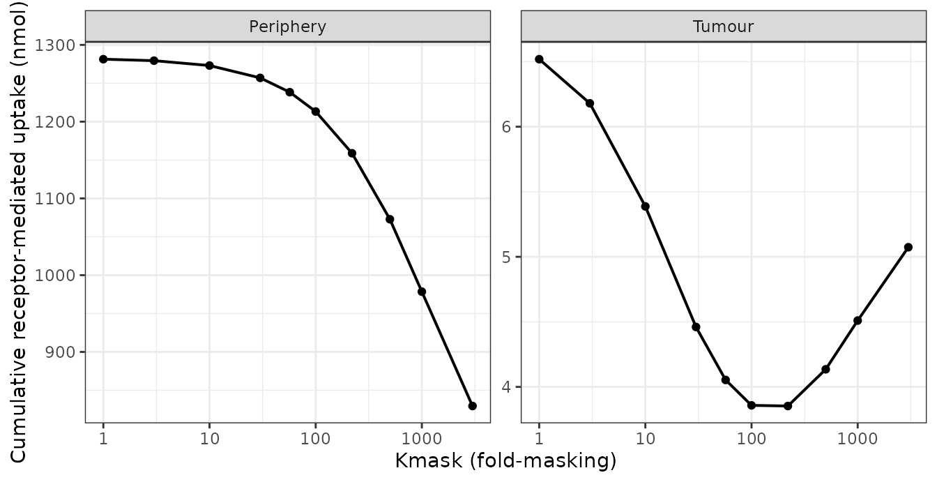
Replicates Figure 4d,e of Stroh 2019: cumulative receptor-mediated uptake at 28 days against mask strength.
Peripheral uptake falls monotonically with mask strength, as Figure 4d reports. Tumour uptake is not monotone – it turns, which is the Results claim, “the relationship of increasing K_mask on receptor-mediated uptake in the tumor is not monotonic and instead may pass through an optimum”. The Discussion sharpens that to a maximum, and this is the one published claim the extraction does not reproduce; see Errata. Splitting the tumour uptake by which kind of arm delivered the molecule to the receptor shows exactly why the curve turns:
humanSummary |>
  dplyr::transmute(
    Kmask = kmask,
    `via open (masked) arm` = signif(uptakeTumourOpen, 3),
    `via cleaved arm` = signif(uptakeTumourCleaved, 3),
    Total = signif(uptakeTumour, 3)
  ) |>
knitr::kable(caption = "Tumour receptor-mediated uptake at 28 days, nmol")| Kmask | via open (masked) arm | via cleaved arm | Total |
|---|---|---|---|
| 1 | 5.5200 | 0.996 | 6.52 |
| 3 | 4.9800 | 1.190 | 6.18 |
| 10 | 3.7400 | 1.650 | 5.39 |
| 30 | 2.2300 | 2.230 | 4.46 |
| 57 | 1.4700 | 2.580 | 4.05 |
| 100 | 0.9740 | 2.880 | 3.86 |
| 220 | 0.5270 | 3.330 | 3.85 |
| 500 | 0.2740 | 3.860 | 4.14 |
| 1000 | 0.1550 | 4.350 | 4.51 |
| 3000 | 0.0599 | 5.010 | 5.07 |
peripheryMonotone <- humanSummary$uptakePeriph[nrow(humanSummary)] <
  humanSummary$uptakePeriph[1]
interiorExtremum <- which.min(humanSummary$uptakeTumour)
tumourNonMonotone <- interiorExtremum > 1L && interiorExtremum < nrow(humanSummary)
c(
  periphery_falls_with_mask = peripheryMonotone,
  tumour_uptake_non_monotone = tumourNonMonotone,
  turning_point_kmask = kmaskGrid[interiorExtremum]
)
#>  periphery_falls_with_mask tumour_uptake_non_monotone
#>                          1                          1
#>        turning_point_kmask
#>                        220
Uptake through a still-masked but transiently open arm falls steadily
as the mask tightens, while uptake through a cleaved arm rises, because
a stronger mask keeps the molecule in circulation long enough for more
of it to be cleaved. The sum of a falling and a rising channel turns
once. Under the Table 2 parameter set the rising channel wins at high
mask strength, so the turn is a minimum near
Kmask = 220.
Human projection: replicating Figure 5
Figure 5 projects circulating total, intact and cleaved Pb-Tx after repeated 3 mg/kg dosing, and concludes that intact Pb-Tx is the majority species.
tau <- 21 * DAY
f5 <- solveMolecule(hu, 220, 3e-7, "pb_c_c_central", 1050,
  times = seq(0, 4 * tau, length.out = 500), tau = tau, nDose = 4L
)
f5 <- dplyr::filter(f5, Cc > 1e-6)

f5 |>
  dplyr::select(time,
    Total = Cc, Intact = pbIntactPlasma, Cleaved = pbCleavedPlasma
  ) |>
  tidyr::pivot_longer(-time, names_to = "species", values_to = "conc") |>
  ggplot2::ggplot(ggplot2::aes(time / DAY, conc, colour = species)) +
  ggplot2::geom_line(linewidth = 0.7) +
  ggplot2::labs(x = "Time (days)", y = "Plasma concentration (nM)", colour = NULL) +
  ggplot2::theme_bw()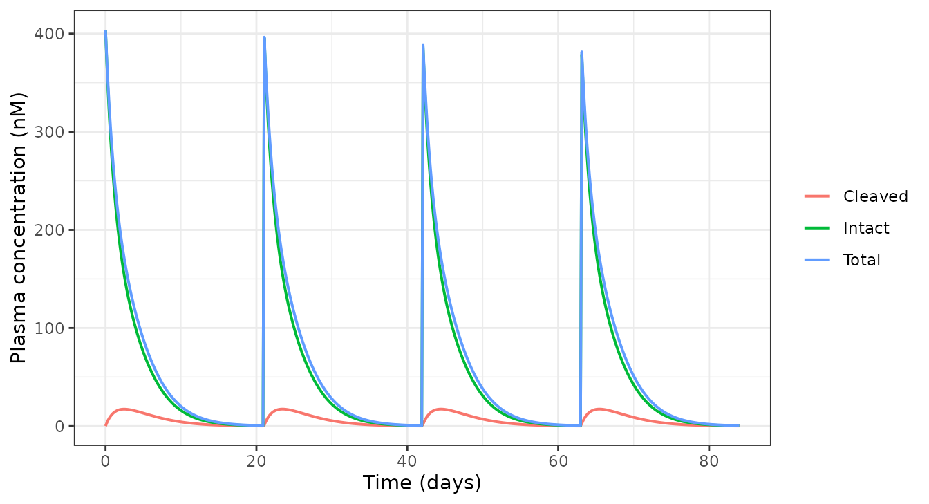
Replicates Figure 5 of Stroh 2019: projected circulating total, intact and cleaved Pb-Tx after repeated dosing.
intactFraction <- f5$pbIntactPlasma / f5$Cc
c(min = min(intactFraction), median = stats::median(intactFraction))
#>       min    median
#> 0.7125151 0.7853998
Intact Pb-Tx never drops below 71 % of circulating drug across four dosing cycles, reproducing “the QSP Pb-Tx model suggests that the intact Pb-Tx comprises the majority of the total circulating species in the plasma”.
Figure S2: cleaved species do not leak back from the tumour
Figure S2 reports that the net flux of cleaved Pb-Tx out of the tumour is at or near zero, which is what makes the tumour-restricted-activation argument work. The flux is computed here from the transport terms directly.
cleavedFree <- c("pb_c_m", "pb_o_m", "pb_m_m")
allFree <- c("pb_c_c", "pb_c_o", "pb_o_o", cleavedFree)
k13 <- exp(hu$iniDf$est[hu$iniDf$name == "lk13"])
k31 <- exp(hu$iniDf$est[hu$iniDf$name == "lk31"])
kelHuman <- exp(hu$iniDf$est[hu$iniDf$name == "lkel"])

netCleavedFlux <-
  k31 * rowSums(hSim[, paste0(cleavedFree, "_tumor"), drop = FALSE]) -
  k13 * rowSums(hSim[, paste0(cleavedFree, "_central"), drop = FALSE])
systemicElim <- kelHuman * rowSums(hSim[, paste0(allFree, "_central"), drop = FALSE])

fluxPct <- 100 * max(abs(netCleavedFlux)) / max(systemicElim)
c(
  max_abs_net_flux_nmol_per_s = max(abs(netCleavedFlux)),
  pct_of_peak_systemic_elimination = fluxPct
)
#>      max_abs_net_flux_nmol_per_s pct_of_peak_systemic_elimination
#>                     8.680742e-07                     8.748544e-02
The largest net efflux of cleaved species from the tumour over the whole profile is 0.087 % of the peak systemic elimination rate – negligible, as Figure S2 reports.
Conclusions
claim <- function(text, pass, achieved, deviation = FALSE) {
  tibble::tibble(Claim = text, Achieved = achieved, Pass = pass, Deviation = deviation)
}
conclusions <- dplyr::bind_rows(
  claim(
    "Model file reproduces the deposited A1 / A2 matrices (54 states)",
    gateRel < 1e-4, sprintf("max relative difference %.2g", gateRel)
  ),
  claim(
    "That gate can go red (0.1 % error in one rate constant)",
    mutRel > 100 * gateRel, sprintf("mutation control %.2g", mutRel)
  ),
  claim(
    "Drug mass balance closes across all species and sinks",
    massErr < 1e-8, sprintf("max relative error %.2g", massErr)
  ),
  claim(
    "CD166 pools start at ksynr / kint; plasma pool and its complexes are zero",
    ssErr < 1e-10 && plasmaBound < 1e-12,
    sprintf("steady-state error %.2g, plasma bound %.2g", ssErr, plasmaBound)
  ),
  claim(
    "Monkey ksynR reproduces Table 1's ~1e4 receptors/cell",
    rpc > 1e3 && rpc < 1e5, sprintf("%.3g receptors/cell", rpc)
  ),
  claim(
    "Figure 3: exposure rises with mask strength, parental mAb lowest",
    orderingHolds, "M1,0 > M1,S1 > M2,S2 > mAb(0,0)"
  ),
  claim(
    "Substrates S1 and S2 are indistinguishable (kcleave constrained equal)",
    substrateIdentical, "identical within dose scaling"
  ),
  claim(
    "TMDD saturates for the parental mAb but not for the masked Pb-Tx",
    parentalRise > 0.4 && maskedRise < 0.1,
    sprintf(
      "AUC/dose rises %.0f %% (parental) vs %.0f %% (masked)",
      100 * parentalRise, 100 * maskedRise
    )
  ),
  claim(
    "Figure 4a,c: plasma and tumour exposure rise with mask strength",
    all(diff(humanSummary$plasmaAuc) > 0) && all(diff(humanSummary$tumourAuc) > 0),
    "monotone increasing over Kmask 1-3000"
  ),
  claim(
    "Figure 4d: peripheral receptor-mediated uptake falls with mask strength",
    peripheryMonotone,
    sprintf(
      "%.0f -> %.0f nmol", humanSummary$uptakePeriph[1],
      humanSummary$uptakePeriph[nrow(humanSummary)]
    )
  ),
  claim(
    "Figure 4e (Results): tumour uptake is non-monotone in mask strength",
    tumourNonMonotone, sprintf("turns at Kmask = %g", kmaskGrid[interiorExtremum])
  ),
  claim(
    "Figure 4e (Discussion): that turning point is a MAXIMUM",
    FALSE, "reproduced as a minimum; see Errata",
    deviation = TRUE
  ),
  claim(
    "Figure 5: intact Pb-Tx is the majority of circulating drug",
    min(intactFraction) > 0.5, sprintf("minimum %.0f %% intact", 100 * min(intactFraction))
  ),
  claim(
    "Figure S2: net flux of cleaved species out of the tumour is ~ zero",
    fluxPct < 1, sprintf("%.2g %% of peak systemic elimination", fluxPct)
  )
)
knitr::kable(conclusions)| Claim | Achieved | Pass | Deviation |
|---|---|---|---|
| Model file reproduces the deposited A1 / A2 matrices (54 states) | max relative difference 3.6e-06 | TRUE | FALSE |
| That gate can go red (0.1 % error in one rate constant) | mutation control 0.016 | TRUE | FALSE |
| Drug mass balance closes across all species and sinks | max relative error 8.4e-13 | TRUE | FALSE |
| CD166 pools start at ksynr / kint; plasma pool and its complexes are zero | steady-state error 2.1e-14, plasma bound 1.7e-20 | TRUE | FALSE |
| Monkey ksynR reproduces Table 1’s ~1e4 receptors/cell | 1.35e+04 receptors/cell | TRUE | FALSE |
| Figure 3: exposure rises with mask strength, parental mAb lowest | M1,0 > M1,S1 > M2,S2 > mAb(0,0) | TRUE | FALSE |
| Substrates S1 and S2 are indistinguishable (kcleave constrained equal) | identical within dose scaling | TRUE | FALSE |
| TMDD saturates for the parental mAb but not for the masked Pb-Tx | AUC/dose rises 66 % (parental) vs 3 % (masked) | TRUE | FALSE |
| Figure 4a,c: plasma and tumour exposure rise with mask strength | monotone increasing over Kmask 1-3000 | TRUE | FALSE |
| Figure 4d: peripheral receptor-mediated uptake falls with mask strength | 1281 -> 830 nmol | TRUE | FALSE |
| Figure 4e (Results): tumour uptake is non-monotone in mask strength | turns at Kmask = 220 | TRUE | FALSE |
| Figure 4e (Discussion): that turning point is a MAXIMUM | reproduced as a minimum; see Errata | FALSE | TRUE |
| Figure 5: intact Pb-Tx is the majority of circulating drug | minimum 71 % intact | TRUE | FALSE |
| Figure S2: net flux of cleaved species out of the tumour is ~ zero | 0.087 % of peak systemic elimination | TRUE | FALSE |
Assumptions, deviations and errata
Source of the ODE system. The article body contains
no equations beyond the generic KroneckerBio form. The entire structure
is taken from Supporting Information PSP4-8-676-s003
(“Model code”), published with the open-access article (PMC6765697). A
copy of its extracted text ships with the package as
inst/references/Stroh_2019_probody_cd166_modelcode.txt so
the structural gate above is reproducible.
kopen is supplement-derived, not
article-derived. Tables 1 and 2 publish only the fold-masking
ratio Kmask. Simulating requires the absolute
breathing timescale, which is recovered from the deposited
A1 entry (3,2) = 2.32e-2 = 2 * kopen, giving
kopen = 1.16e-2 /s, and is independently corroborated by
Ippolito 2024 Table S2 citing Stroh 2019 for the same number.
The deposited matrices are not the Table 2 parameter
set. The deposited instance uses Kmask = 20,
kcleave = 1e-6 /s (above the article’s stated
< 3e-7 bound), k13 = 2.5e-9 and
k31 = 4.4e-6 /s (Table 2 gives 1.9e-8 and
1.0e-5). It is evidently one point from the parameter scans
the paper reports rather than the published human parameterisation. The
model files therefore carry the Table 2 / Table 1 published
values, and the deposited instance is used only in the
structural gate, where the parameter values are irrelevant to what is
being tested.
k_off1: the printed formula omits a factor of
two. Table 1 gives k off1 = k on1 * K app with
k on1 = 1e-3 and K app = 1.0 nM, which
evaluates to 1e-3, but the tabulated value is
2e-3. The deposited A1 matrix uses
2e-3 throughout (entries (1,8),
(1,9), (1,11) and so on). Two independent
sources therefore carry 2e-3 against one printed relation,
and K app is an apparent (bivalent) affinity whose
relation to the monovalent off-rate legitimately carries a statistical
factor of two for a two-armed molecule. The extraction uses
2e-3.
Plasma CD166 is carried but never synthesised. The
deposited code gives the plasma compartment a full complement of
receptor and bound states, but Figure 2b draws no CD166 in plasma and
the Results say provisions were included “for binding to target within
the peripheral and tumor compartments”. The extraction sets
ksynr_central to a fixed zero, which makes the plasma block
inert (verified above at 1.7^{-20} nmol) while keeping the state
indexing identical to the deposit. A user who wants to model soluble
plasma CD166 can simply raise that one parameter.
pb_el_tumor is omitted. The deposited
state list names it, but A1 gives it no influx, because
free species in the tumour are not eliminated. It would be an
identically-zero state, so the model file carries 54 live states rather
than 55.
No tumour compartment in the monkey model. Table 1 reports no tumour volume, perfusion rate or partition coefficient, and the animals were experimentally naive rather than tumour-bearing. The monkey model is therefore plasma plus periphery. Every tumour parameter in the human model comes from Table 2.
Doses are entered in nmol, not mg/kg. The paper
never reports the Pb-Tx molecular weight, so mg/kg cannot be converted
to a molar amount from any available source, and substituting a
class-typical antibody mass would be a guess. The simulations above
instead dose the molar amounts that place the 10 mg/kg monkey arm near
the ~1.3e3 nM initial level of Figure 3c, scaling the other
arms proportionally. This is a presentation choice for the figures only:
every assertion in the Conclusions table is a ratio, an ordering, a mass
balance or a structural identity, so none of them depends on it.
Deviation – Figure 4e curvature. The Results
describe tumour receptor-mediated uptake as “not monotonic and instead
may pass through an optimum”, which is reproduced. The Discussion
sharpens this to “concave-down and pass through a maxima”, which is
not reproduced: under the Table 2 parameter set, and
under every alternative sourced from the paper that was tried (no
cleavage; 100-fold rather than 10-fold tumour kcleave; the
deposited instance), the turning point is a minimum. The
decomposition table above shows the mechanism: uptake via a still-masked
open arm falls monotonically with Kmask (5.5 to 0.06 nmol)
while uptake via a cleaved arm rises monotonically (1.0 to 5.0 nmol),
and a falling plus a rising channel gives a minimum. Obtaining the
published maximum would require the total tumour Pb-Tx amount to grow
faster with Kmask than the open fraction shrinks over the
low-to-mid range, and here it does not – tumour exposure rises about
eight-fold across the scan while the open fraction falls roughly as
1/Kmask. The published Figure 4e was produced with an
unstated Kmask grid and, as noted above, the deposited code
does not carry the Table 2 values, so the disagreement cannot be
resolved from the available sources. It is recorded here rather than
tuned away.
No variability. The source model is deterministic:
no between-subject variability and no residual-error model are reported,
and none is invented. Both model files therefore carry no
eta terms and no error model, and rxSolve is
called without omega.
Unit note on the bimolecular terms. Table 1’s own
receptors-per-cell arithmetic
(RPC = k_synR / k_endo * 1e-9 * Avog / Ncell) shows that
ksynr / kint is an amount in nmol, so the states
are amounts. The tabulated k_on values are nevertheless
labelled 1/(nM*second) and are used in the deposited
matrices without any volume division. The extraction reproduces the
deposited arithmetic exactly and flags the labelling inconsistency here
rather than silently rescaling it, which would change the model.