Afabicin in vitro to in vivo translation against Staphylococcus aureus (Saporta 2024)
Source:vignettes/articles/Saporta_2024_afabicin.Rmd
Saporta_2024_afabicin.RmdModel and source
Saporta 2024 built a semi-mechanistic pharmacokinetic/pharmacodynamic (PK/PD) model of afabicin desphosphono, the active moiety of the FabI-inhibitor prodrug afabicin, on static in vitro time-kill data from 21 Staphylococcus aureus strains. They then re-estimated it jointly on those data and on neutropenic mouse thigh infection data from 9 strains. The paper reports both parameter sets (Table 1), and each is packaged as its own model file.
mod_invitro <- rxode2::rxode(readModelDb("Saporta_2024_afabicin_invitro"))
mod_joint <- rxode2::rxode(readModelDb("Saporta_2024_afabicin_invitro_mouse"))

# Typical-value versions: the models have no inter-experiment variability, so
# only the residual error is zeroed.
mod_invitro_tv <- rxode2::zeroRe(mod_invitro, "sigma")
mod_joint_tv <- rxode2::zeroRe(mod_joint, "sigma")

# With no omega, rxode2 notes that a multi-subject solve has no between-subject
# variability. That is expected here and is muffled; any other warning shows.
muffle_no_omega <- function(w) {
  if (grepl("multi-subject simulation without", conditionMessage(w))) {
    invokeRestart("muffleWarning")
  }
}
solve_df <- function(model, ev, ...) {
  withCallingHandlers(
    as.data.frame(rxode2::rxSolve(model, ev, ...)),
    warning = muffle_no_omega
  )
}- Citation: Saporta R, Nielsen EI, Menetrey A, Cameron DR, Nicolas-Metral V, Friberg LE. Model-based translation of results from in vitro to in vivo experiments for afabicin activity against Staphylococcus aureus. J Antimicrob Chemother. 2024;79(12):3150-3159. doi:10.1093/jac/dkae334. PMID: 39315768. PMCID: PMC11638087. Model structure: Materials and methods, Eqs 1-6, and Figure 1. Parameter estimates: Table 1, column ‘PK/PD model based on in vitro data’. Strain MICs: Supplementary Table S1. kdeath fixed to 0.179 per hour from Nielsen EI et al., Antimicrob Agents Chemother 2007;51:128-136; koff fixed to 0.0139 per hour from Mohamed AF et al., Antimicrob Agents Chemother 2012;56:179-188.
- Article: https://doi.org/10.1093/jac/dkae334
- PubMed Central open-access copy: https://pmc.ncbi.nlm.nih.gov/articles/PMC11638087/
| Model file | Role |
|---|---|
Saporta_2024_afabicin_invitro |
Fit to the 162 in vitro time-kill curves alone (Table 1, first estimate column) |
Saporta_2024_afabicin_invitro_mouse |
Joint re-estimation on the in vitro and neutropenic mouse thigh data (Table 1, second estimate column); carries an in vitro system and a thigh system side by side |
Structure
Source Figure 1 and Equations 1-6. Bacteria are either growing and
drug-susceptible (S) or dormant and drug-insusceptible
(D):
dS/dt = kgrowth * S - (kdeath + kdrug) * S - kSD * SdD/dt = kSD * S - kdeath * D-
kSD = (S + D) * (kgrowth - kdeath) / Bmax, which brings the total count toBmaxat stationary phase.
Afabicin desphosphono adds a sigmoid Emax killing rate on
S,
kdrug = Emax(t) * C^Hill / (EC50^Hill + C^Hill), where
C is the unbound concentration. The strain MIC scales EC50
as EC50 = beta * MIC^gamma, with beta fixed to
1 in vitro. A reversible adaptation pair, ASoff and ASon
(aroff and aron in the model), starts at ASoff
= 1. Drug drives the transfer to ASon at rate kon * C, and
bacteria return at koff. Adaptation reduces the maximum
effect as Emax(t) = Emax * (1 - ASon / (ASon + AS50)).
In the joint model, kgrowth, kdeath,
Emax, gamma, Hill,
kon, koff and AS50 are shared
between settings. Bmax, beta and the residual
error are setting-specific. The thigh system is driven by the unbound
plasma concentration fu * CP_AFABICIN_DESPHOSPHONO_MGL,
with fu = 0.02.
The mouse PK is a user-supplied input
Saporta 2024 derived the mouse plasma concentrations from the
afabicin mouse PK model of Bader 2017, which was presented only as a
conference poster (ASM Microbe 2017, abstract 2176). Supplementary text
2 of the follow-up paper Saporta 2026 (https://doi.org/10.1128/aac.00959-25) prints its
structure: an intraperitoneal depot and absorption transit compartment
feeding a two-compartment afabicin desphosphono model through an
afabicin-to-desphosphono conversion factor. No published source gives
its parameter values. The joint model therefore takes the total afabicin
desphosphono plasma concentration as a time-varying covariate column,
CP_AFABICIN_DESPHOSPHONO_MGL (mg/L), and applies the
paper’s unbound fraction inside the model. To simulate a dosing regimen,
a user supplies that column from a mouse PK model of their choice. For
the same reason, this article cannot replicate the dose-response panels
of source Figures 3 and 4.
Population
str(mod_joint$population, max.level = 1)
#> List of 9
#>  $ species       : chr "in vitro (Staphylococcus aureus) + mouse (female ICR or Swiss Webster, neutropenic)"
#>  $ n_subjects    : int 952
#>  $ n_studies     : int NA
#>  $ organism      : chr "Staphylococcus aureus: 21 strains in vitro (MIC 0.004 to 0.03 mg/L) and 9 strains in vivo (6 MRSA; MIC 0.004 to"| __truncated__
#>  $ system        : chr "In vitro: 162 static time-kill curves in Mueller-Hinton Broth II at 35 C (722 counts). In vivo: neutropenic mou"| __truncated__
#>  $ dose_range    : chr "Afabicin (prodrug) started 2 h after infection: a single 129 mg/kg dose, or 0.011 to 190 mg/kg every 6 h, given"| __truncated__
#>  $ sex_female_pct: num 100
#>  $ disease_state : chr "Neutropenic thigh infection with Staphylococcus aureus (in vivo arm)"
#>  $ notes         : chr "n_subjects counts the mice (568 ICR, 384 Swiss Webster); the in vitro arm adds 162 time-kill curves. The bacter"| __truncated__
In vitro. 162 static time-kill curves (722 counts, 8 of them below the 200 CFU/mL limit of detection) from 21 S. aureus strains, 12 of them MRSA. Afabicin desphosphono MICs ranged from 0.004 to 0.03 mg/L (Supplementary Table S1), and concentrations from 0.004 to 1 mg/L plus drug-free growth controls. Experiments ran in Mueller-Hinton Broth II at 35 C, with target inocula of 1.6e5 to 2.0e7 CFU/mL, sampled up to 24 or 48 h.
In vivo. 952 female ICR or Swiss Webster mice, rendered neutropenic with cyclophosphamide (150 mg/kg on Day -4 and 100 mg/kg on Day -1). The left thigh was infected with 8.0e4 to 1.3e7 CFU of one of 9 strains (MIC 0.004 to 0.06 mg/L), and treatment started 2 h after infection. Afabicin was given as a single 129 mg/kg dose or as 0.011 to 190 mg/kg every 6 h, IV (n = 82) or IP (n = 430). Thighs were harvested at 2, 26, 50 or 74 h after infection. Only S. aureus ATCC 29213 was studied both in vitro and in vivo, so it is the default strain (MIC 0.008 mg/L) in both model files.
Source trace
Every ini() entry carries an in-file comment naming its
source location.
Equations
| Equation | Source location |
|---|---|
dS/dt, dD/dt
|
Materials and methods, Eqs 1-2; Figure 1 |
kSD = (S + D) * (kgrowth - kdeath) / Bmax |
Materials and methods, sentence after Eq 2 |
dASoff/dt, dASon/dt, initial ASoff = 1,
ASon = 0 |
Eqs 3-4 and the sentence before them |
Emax(t) = Emax * (1 - ASon / (ASon + AS50)) |
Eq 5 |
EC50 = beta * MIC^gamma, beta fixed to 1
in vitro |
Eq 6; Results, “PK/PD model for in vitro data” |
Sigmoid Emax kdrug
|
Results: “Afabicin desphosphono effect was implemented as a sigmoid
Emax function”; Table 1 Hill row |
All bacteria start in S
|
Materials and methods, “PK/PD model for in vitro data” |
Setting-specific Bmax, beta, residual
error; shared others |
Methods and Results, “PK/PD model for in vivo data” |
Thigh driven by unbound concentration, fu = 0.02
|
Methods, “PK/PD model for in vivo data” |
| Log10 counts, additive error | Methods, “Data analysis and software”; Table 1 footnote b |
Parameters
| Parameter | In vitro file | Joint file | Source location |
|---|---|---|---|
lkgrowth |
log(1.13) FIXED | log(1.10) FIXED | Table 1 kgrowth; footnote a (fixed from the
growth-control fit) |
lkdeath |
log(0.179) FIXED | log(0.179) FIXED | Table 1 kdeath; literature value, Nielsen 2007 |
lbmax |
log(10^9.85) FIXED | log(10^9.86) FIXED | Table 1 Bmax vitro; footnote a |
lbmax_thigh |
– | log(10^9.08) FIXED | Table 1 Bmax vivo; footnote a |
lemax |
log(4.10) | log(3.37) | Table 1 Emax
|
lec50 (beta in vitro) |
log(1) FIXED | log(1) FIXED | Table 1 beta vitro
|
lec50_thigh (beta in vivo) |
– | log(0.707) | Table 1 beta vivo
|
e_mic_ec50 (gamma) |
0.160 | 0.204 | Table 1 gamma
|
lhill |
log(0.360) | log(0.324) | Table 1 Hill
|
lkon |
log(0.406) | log(0.386) | Table 1 kon, mL/(ug h) = L/(mg h) |
lkoff |
log(0.0139) FIXED | log(0.0139) FIXED | Table 1 koff; 50 h half-life from Mohamed 2012 |
lar50 (AS50) |
log(0.861) | log(1.18) | Table 1 AS50
|
addSd / addSd_log_cfu_invitro
|
0.869 | 0.877 | Table 1 RES vitro
|
addSd_log_cfu_thigh |
– | 0.621 | Table 1 RES vivo
|
fu |
– | 0.02 FIXED | Methods, “PK/PD model for in vivo data” |
mic, mic_thigh
|
0.008 FIXED | 0.008 FIXED | Supplementary Table S1 (ATCC 29213); design input |
linoc, linoc_thigh
|
log(1e6) FIXED | log(1e6) FIXED | Design input; Figure 2 median starting inoculum about 6 log10 CFU/mL |
Checks against values stated in the text
Several derived quantities are printed in the Results and Discussion. The model reproduces them exactly from the Table 1 estimates:
ec50_at <- function(beta, gamma, mic) beta * mic^gamma
emax_adapted <- function(emax, as50) emax * (1 - 1 / (1 + as50))

chk <- tibble::tribble(
  ~quantity, ~paper, ~model,
  "In vitro EC50 at MIC 0.008 (mg/L)", 0.46, ec50_at(1, 0.160, 0.008),
  "In vitro EC50 at MIC 0.03 (mg/L)", 0.57, ec50_at(1, 0.160, 0.03),
  "In vivo EC50 at MIC 0.004 (mg/L)", 0.23, ec50_at(0.707, 0.204, 0.004),
  "In vivo EC50 at MIC 0.008 (mg/L)", 0.26, ec50_at(0.707, 0.204, 0.008),
  "In vivo EC50 at MIC 0.03 (mg/L)", 0.35, ec50_at(0.707, 0.204, 0.03),
  "EC50 ratio when MIC doubles, in vitro", 1.12, 2^0.160,
  "Emax reduction at full adaptation, in vitro (fraction)", 0.54, 1 / (1 + 0.861),
  "kdrug ceiling at full adaptation, in vitro (1/h)", 1.89, emax_adapted(4.10, 0.861),
  "kdrug ceiling at full adaptation, in vivo (1/h)", 1.82, emax_adapted(3.37, 1.18)
) |>
  mutate(pct_diff = 100 * (model - paper) / paper)

chk |>
  mutate(model = signif(model, 3), pct_diff = round(pct_diff, 1)) |>
  rename(Quantity = quantity, Paper = paper, Model = model, "% difference" = pct_diff) |>
knitr::kable()| Quantity | Paper | Model | % difference |
|---|---|---|---|
| In vitro EC50 at MIC 0.008 (mg/L) | 0.46 | 0.462 | 0.4 |
| In vitro EC50 at MIC 0.03 (mg/L) | 0.57 | 0.571 | 0.1 |
| In vivo EC50 at MIC 0.004 (mg/L) | 0.23 | 0.229 | -0.3 |
| In vivo EC50 at MIC 0.008 (mg/L) | 0.26 | 0.264 | 1.5 |
| In vivo EC50 at MIC 0.03 (mg/L) | 0.35 | 0.346 | -1.2 |
| EC50 ratio when MIC doubles, in vitro | 1.12 | 1.120 | -0.2 |
| Emax reduction at full adaptation, in vitro (fraction) | 0.54 | 0.537 | -0.5 |
| kdrug ceiling at full adaptation, in vitro (1/h) | 1.89 | 1.900 | 0.4 |
| kdrug ceiling at full adaptation, in vivo (1/h) | 1.82 | 1.820 | 0.2 |
# The paper rounds to two significant figures, so a few percent is rounding.
stopifnot(all(abs(chk$pct_diff) < 5))
The Results also state that the in vivo EC50 was “38% to 45% lower within the studied MIC range” than in vitro. Across the in vivo MIC range of 0.004 to 0.06 mg/L, the ratio of the two Eq 6 curves gives:
Growth controls reach Bmax
Without drug, both systems must plateau at their tabulated
Bmax: 9.85 log10 CFU/mL for the in vitro fit, and 9.86
log10 CFU/mL and 9.08 log10 CFU/g for the two systems of the joint
fit.
obs_times <- c(0, 2, 6, 12, 24, 48, 74)

ev_vitro_ctrl <- rxode2::et(obs_times, cmt = "bact_s")
gc_vitro <- solve_df(mod_invitro_tv, ev_vitro_ctrl)

ev_joint_ctrl <- data.frame(
  id = 1L, time = obs_times, evid = 0L, dvid = 1L,
  CP_AFABICIN_DESPHOSPHONO_MGL = 0
)
gc_joint <- solve_df(mod_joint_tv, ev_joint_ctrl)

plateau <- c(
  invitro = gc_vitro$log_cfu[gc_vitro$time == 74],
  joint_invitro = gc_joint$log_cfu_invitro[gc_joint$time == 74],
  joint_thigh = gc_joint$log_cfu_thigh[gc_joint$time == 74]
)
round(plateau, 3)
#>       invitro joint_invitro   joint_thigh
#>         9.851         9.860         9.081
stopifnot(
  abs(plateau[["invitro"]] - 9.85) < 0.02,
  abs(plateau[["joint_invitro"]] - 9.86) < 0.02,
  abs(plateau[["joint_thigh"]] - 9.08) < 0.02
)
Replicate Figure 2 (in vitro time-kill VPC)
Source Figure 2 shows, for every combination of concentration and MIC, the median of simulated counts (solid line). The maintainers digitised the median line of all 30 panels at 24 h and, where the panel runs that long, at 48 h. They also recorded the value where the line starts, which stands in for that panel’s starting inoculum.
The line usually starts at the first sampling time, close to 0 h. For four sparse panels (the three MIC 0.03 mg/L panels and 0.064 mg/L at MIC 0.004 mg/L), the first sample is at 6 h. For these, the simulation starts at time zero from the median starting inoculum drawn as the upper broken line, about 6.2 log10 CFU/mL, and the 6 h value is compared too. The typical-value simulation below uses the in vitro model unchanged.
fig2 <- tibble::tribble(
  ~conc, ~mic, ~start_time, ~start_value, ~t6, ~t24, ~t48,
  0,     0.004, 0, 9.2, NA,  10.0, 10.0,
  0,     0.008, 0, 6.8, NA,  9.8,  NA,
  0,     0.015, 0, 6.6, NA,  9.8,  9.9,
  0,     0.03,  0, 8.6, NA,  10.0, 10.0,
  0.004, 0.004, 0, 7.0, NA,  9.4,  9.4,
  0.008, 0.008, 0, 7.3, NA,  9.1,  NA,
  0.015, 0.008, 0, 6.0, NA,  7.0,  8.4,
  0.015, 0.015, 0, 6.8, NA,  8.3,  9.2,
  0.016, 0.004, 0, 6.3, NA,  7.2,  8.5,
  0.03,  0.008, 0, 6.3, NA,  5.8,  6.7,
  0.03,  0.015, 0, 5.9, NA,  6.0,  7.3,
  0.032, 0.008, 0, 6.2, NA,  5.8,  NA,
  0.06,  0.008, 0, 5.8, NA,  4.6,  NA,
  0.06,  0.015, 0, 6.5, NA,  5.3,  6.4,
  0.06,  0.03,  6, 6.2, 5.4, 5.4,  6.7,
  0.064, 0.004, 6, 6.2, 5.8, 5.2,  5.8,
  0.12,  0.008, 0, 5.5, NA,  4.0,  5.0,
  0.12,  0.03,  6, 6.2, 5.2, 5.0,  6.2,
  0.128, 0.008, 0, 6.3, NA,  4.3,  NA,
  0.13,  0.008, 0, 5.9, NA,  4.2,  NA,
  0.15,  0.008, 0, 6.0, NA,  4.3,  NA,
  0.24,  0.015, 0, 5.8, NA,  5.0,  5.7,
  0.25,  0.008, 0, 5.8, NA,  3.9,  NA,
  0.25,  0.015, 0, 6.0, NA,  4.8,  5.2,
  0.32,  0.008, 0, 6.5, NA,  5.5,  NA,
  0.5,   0.008, 0, 5.6, NA,  3.8,  NA,
  0.5,   0.03,  6, 6.2, 5.0, 4.6,  4.5,
  0.6,   0.008, 0, 5.9, NA,  3.8,  NA,
  0.96,  0.015, 0, 5.8, NA,  3.7,  NA,
  1,     0.008, 0, 6.0, NA,  3.7,  NA
) |>
  mutate(
    id = row_number(),
    panel = sprintf("%g | MIC %g", conc, mic)
  )
fig2_times <- seq(0, 48, by = 1)
ev_fig2 <- bind_rows(
  fig2 |>
    transmute(id, time = 0, evid = 1L, amt = conc, cmt = "afabicin_desphosphono"),
  tidyr::expand_grid(id = fig2$id, time = fig2_times) |>
    mutate(evid = 0L, amt = 0, cmt = "bact_s")
) |>
  arrange(id, time, desc(evid))

params_fig2 <- fig2 |>
  transmute(id, mic, linoc = log(10^start_value))

sim_fig2 <- solve_df(mod_invitro_tv, ev_fig2, params = params_fig2) |>
  left_join(fig2 |> select(id, panel), by = "id")
fig2_points <- fig2 |>
  select(panel, t6, t24, t48) |>
  pivot_longer(c(t6, t24, t48), names_to = "time", values_to = "log_cfu") |>
  filter(!is.na(log_cfu)) |>
  mutate(time = as.numeric(sub("t", "", time)))

ggplot(sim_fig2, aes(time, log_cfu)) +
  geom_line() +
  geom_point(data = fig2_points, colour = "firebrick", size = 2) +
  geom_hline(yintercept = log10(200), linetype = "dashed", colour = "grey50") +
  facet_wrap(~panel, ncol = 5) +
  scale_x_continuous(breaks = c(0, 12, 24, 36, 48)) +
  labs(x = "Time (h)", y = "Bacterial count (log10 CFU/mL)")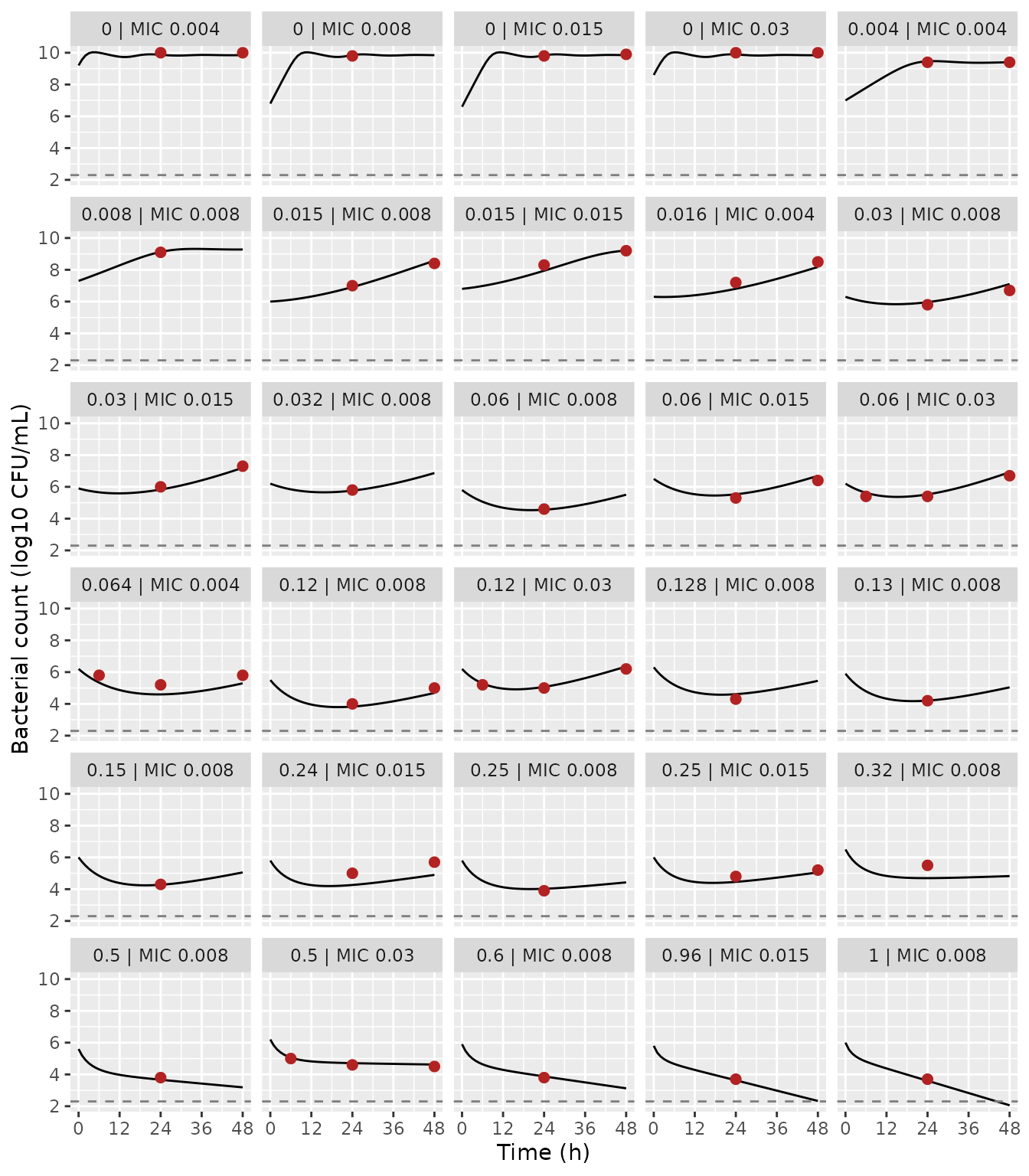
Replicates Figure 2 of Saporta 2024: typical-value in vitro time-kill curves (lines) against the median simulated counts digitised from the source figure (points). Broken lines: 200 CFU/mL limit of detection.
fig2_cmp <- fig2_points |>
  inner_join(sim_fig2 |> select(panel, time, sim = log_cfu), by = c("panel", "time")) |>
  mutate(diff = sim - log_cfu)

fig2_cmp |>
  mutate(sim = round(sim, 2), diff = round(diff, 2)) |>
  rename(
    Panel = panel, "Time (h)" = time, "Figure 2 median (log10)" = log_cfu,
    "Model (log10)" = sim, "Difference (log10)" = diff
  ) |>
knitr::kable()| Panel | Time (h) | Figure 2 median (log10) | Model (log10) | Difference (log10) |
|---|---|---|---|---|
| 0 | MIC 0.004 | 24 | 10.0 | 9.87 | -0.13 |
| 0 | MIC 0.004 | 48 | 10.0 | 9.85 | -0.15 |
| 0 | MIC 0.008 | 24 | 9.8 | 9.85 | 0.05 |
| 0 | MIC 0.015 | 24 | 9.8 | 9.83 | 0.03 |
| 0 | MIC 0.015 | 48 | 9.9 | 9.85 | -0.05 |
| 0 | MIC 0.03 | 24 | 10.0 | 9.89 | -0.11 |
| 0 | MIC 0.03 | 48 | 10.0 | 9.85 | -0.15 |
| 0.004 | MIC 0.004 | 24 | 9.4 | 9.46 | 0.06 |
| 0.004 | MIC 0.004 | 48 | 9.4 | 9.40 | 0.00 |
| 0.008 | MIC 0.008 | 24 | 9.1 | 9.12 | 0.02 |
| 0.015 | MIC 0.008 | 24 | 7.0 | 6.91 | -0.09 |
| 0.015 | MIC 0.008 | 48 | 8.4 | 8.57 | 0.17 |
| 0.015 | MIC 0.015 | 24 | 8.3 | 7.94 | -0.36 |
| 0.015 | MIC 0.015 | 48 | 9.2 | 9.21 | 0.01 |
| 0.016 | MIC 0.004 | 24 | 7.2 | 6.81 | -0.39 |
| 0.016 | MIC 0.004 | 48 | 8.5 | 8.17 | -0.33 |
| 0.03 | MIC 0.008 | 24 | 5.8 | 5.96 | 0.16 |
| 0.03 | MIC 0.008 | 48 | 6.7 | 7.10 | 0.40 |
| 0.03 | MIC 0.015 | 24 | 6.0 | 5.83 | -0.17 |
| 0.03 | MIC 0.015 | 48 | 7.3 | 7.20 | -0.10 |
| 0.032 | MIC 0.008 | 24 | 5.8 | 5.76 | -0.04 |
| 0.06 | MIC 0.008 | 24 | 4.6 | 4.56 | -0.04 |
| 0.06 | MIC 0.015 | 24 | 5.3 | 5.53 | 0.23 |
| 0.06 | MIC 0.015 | 48 | 6.4 | 6.69 | 0.29 |
| 0.06 | MIC 0.03 | 6 | 5.4 | 5.63 | 0.23 |
| 0.06 | MIC 0.03 | 24 | 5.4 | 5.53 | 0.13 |
| 0.06 | MIC 0.03 | 48 | 6.7 | 6.92 | 0.22 |
| 0.064 | MIC 0.004 | 6 | 5.8 | 5.34 | -0.46 |
| 0.064 | MIC 0.004 | 24 | 5.2 | 4.60 | -0.60 |
| 0.064 | MIC 0.004 | 48 | 5.8 | 5.29 | -0.51 |
| 0.12 | MIC 0.008 | 24 | 4.0 | 3.83 | -0.17 |
| 0.12 | MIC 0.008 | 48 | 5.0 | 4.69 | -0.31 |
| 0.12 | MIC 0.03 | 6 | 5.2 | 5.29 | 0.09 |
| 0.12 | MIC 0.03 | 24 | 5.0 | 5.07 | 0.07 |
| 0.12 | MIC 0.03 | 48 | 6.2 | 6.35 | 0.15 |
| 0.128 | MIC 0.008 | 24 | 4.3 | 4.61 | 0.31 |
| 0.13 | MIC 0.008 | 24 | 4.2 | 4.21 | 0.01 |
| 0.15 | MIC 0.008 | 24 | 4.3 | 4.28 | -0.02 |
| 0.24 | MIC 0.015 | 24 | 5.0 | 4.26 | -0.74 |
| 0.24 | MIC 0.015 | 48 | 5.7 | 4.90 | -0.80 |
| 0.25 | MIC 0.008 | 24 | 3.9 | 4.02 | 0.12 |
| 0.25 | MIC 0.015 | 24 | 4.8 | 4.46 | -0.34 |
| 0.25 | MIC 0.015 | 48 | 5.2 | 5.05 | -0.15 |
| 0.32 | MIC 0.008 | 24 | 5.5 | 4.69 | -0.81 |
| 0.5 | MIC 0.008 | 24 | 3.8 | 3.67 | -0.13 |
| 0.5 | MIC 0.03 | 6 | 5.0 | 5.06 | 0.06 |
| 0.5 | MIC 0.03 | 24 | 4.6 | 4.71 | 0.11 |
| 0.5 | MIC 0.03 | 48 | 4.5 | 4.62 | 0.12 |
| 0.6 | MIC 0.008 | 24 | 3.8 | 3.88 | 0.08 |
| 0.96 | MIC 0.015 | 24 | 3.7 | 3.63 | -0.07 |
| 1 | MIC 0.008 | 24 | 3.7 | 3.60 | -0.10 |
stopifnot(
  # Every digitised value found its simulated time point.
  nrow(fig2_cmp) == sum(!is.na(c(fig2$t6, fig2$t24, fig2$t48))),
  # A mis-transcribed Emax, EC50 power or Hill factor shifts most panels by
  # more than a log10; digitising a median line is good to about 0.3 log10.
  median(abs(fig2_cmp$diff)) < 0.3,
  # The paper's own yardstick for an adequate prediction is +/- 1 log10.
  max(abs(fig2_cmp$diff)) < 1
)
Most panels agree within a few tenths of a log10. The largest differences, up to about 0.8 log10, are in sparse panels where the model kills somewhat faster than the source median line: 0.24 mg/L at MIC 0.015, 0.32 mg/L at MIC 0.008, and 0.064 mg/L at MIC 0.004. In each of them the starting inoculum is read off the figure or assumed, and the later counts move with it one-for-one. The source medians were simulated from each experiment’s own design, which is not published.
Simulated observations for one condition
A stochastic simulation adds the additive log10 residual error, 0.869 log10 CFU/mL, to the typical curve. Here it is shown for 0.12 mg/L against an MIC 0.008 mg/L strain, a condition that shows both early killing and adaptation-driven regrowth. The paper’s grey band is a confidence interval of the median, not a prediction interval. So the comparison here is limited to the median, which stays on the digitised line.
rxode2::rxSetSeed(20241)
n_rep <- 200L
ev_vpc <- bind_rows(
  tibble(id = seq_len(n_rep), time = 0, evid = 1L, amt = 0.12, cmt = "afabicin_desphosphono"),
  tidyr::expand_grid(id = seq_len(n_rep), time = c(0, 2, 4, 6, 8, 12, 24, 30, 36, 48)) |>
    mutate(evid = 0L, amt = 0, cmt = "bact_s")
) |>
  arrange(id, time, desc(evid))

sim_vpc <- solve_df(
  mod_invitro, ev_vpc,
  params = c(mic = 0.008, linoc = log(10^5.5))
)

vpc_sum <- sim_vpc |>
  group_by(time) |>
  summarise(
    median = median(sim),
    lo = quantile(sim, 0.05),
    hi = quantile(sim, 0.95),
    .groups = "drop"
  )
ggplot(vpc_sum, aes(time, median)) +
  geom_ribbon(aes(ymin = lo, ymax = hi), fill = "grey80") +
  geom_line() +
  geom_point(
    data = fig2_points |> filter(panel == "0.12 | MIC 0.008"),
    aes(time, log_cfu), colour = "firebrick", size = 2
  ) +
  labs(x = "Time (h)", y = "Bacterial count (log10 CFU/mL)")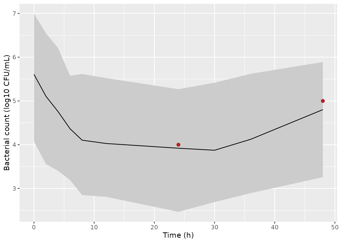
Simulated observations (median and 90% prediction interval) for 0.12 mg/L afabicin desphosphono against an MIC 0.008 mg/L strain; points are the median line digitised from the matching panel of source Figure 2.
In vitro and in vivo parameter sets in the thigh
The joint model’s thigh system can be solved under a constant unbound
concentration without a mouse PK model, by holding the covariate fixed.
That isolates the pharmacodynamic difference the paper reports. The
re-estimated in vivo beta of 0.707 lowers EC50 by about
40%. The in vitro estimates (Table 1, first column), run with the in
vivo growth parameters (kgrowth 1.10 /h, Bmax
9.08 log10 CFU/g), give the “prediction” scenario of source Figure 3.
The unbound concentrations below bracket the EC50 at an MIC of 0.008
mg/L, which is 0.26 mg/L in vivo and 0.46 mg/L in vitro.
cu_levels <- c(0.03, 0.1, 0.3, 1, 3)
thigh_times <- seq(0, 74, by = 1)

ev_thigh <- tidyr::expand_grid(
  id = seq_along(cu_levels), time = thigh_times
) |>
  mutate(
    evid = 0L, dvid = 2L,
    cu = cu_levels[id],
    CP_AFABICIN_DESPHOSPHONO_MGL = ifelse(time >= 2, cu / 0.02, 0)
  )

# The in vitro drug-effect estimates (Table 1, first column) with the in vivo
# growth parameters, as in the source "Prediction of in vivo efficacy" step.
params_invitro_pred <- c(
  lemax = log(4.10), lec50_thigh = log(1), e_mic_ec50 = 0.160,
  lhill = log(0.360), lkon = log(0.406), lar50 = log(0.861)
)

sim_thigh <- bind_rows(
  solve_df(mod_joint_tv, ev_thigh, keep = "cu") |>
    mutate(parameters = "Joint re-estimation (in vivo beta = 0.707)"),
  solve_df(mod_joint_tv, ev_thigh, params = params_invitro_pred, keep = "cu") |>
    mutate(parameters = "In vitro estimates (prediction)")
) |>
  mutate(exposure = sprintf("Unbound C = %g mg/L from 2 h", cu))
ggplot(sim_thigh, aes(time, log_cfu_thigh, colour = parameters)) +
  geom_line() +
  facet_wrap(~exposure) +
  labs(x = "Time after infection (h)", y = "Thigh count (log10 CFU/g)", colour = NULL) +
  theme(legend.position = "bottom")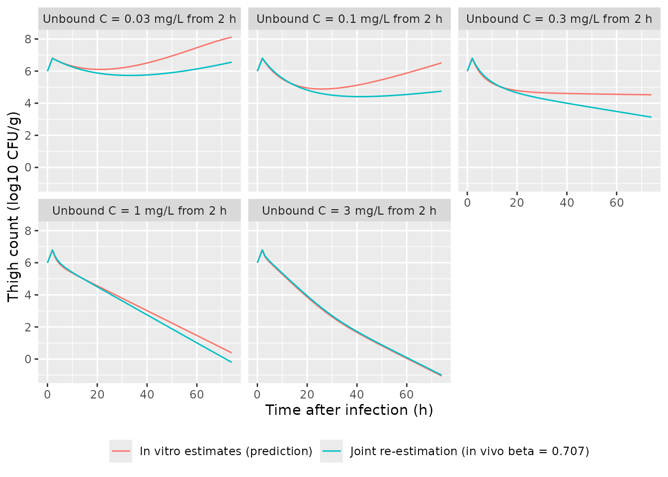
Thigh bacterial counts (MIC 0.008 mg/L, 6 log10 CFU/g at infection) under constant unbound afabicin desphosphono concentrations started 2 h after infection, with the jointly re-estimated parameters and with the in vitro estimates. Constant exposure is illustrative; it is not an afabicin dosing regimen.
thigh_tab <- sim_thigh |>
  filter(time %in% c(26, 74)) |>
  select(cu, time, parameters, log_cfu_thigh) |>
  pivot_wider(names_from = parameters, values_from = log_cfu_thigh) |>
  mutate(
    difference = `Joint re-estimation (in vivo beta = 0.707)` -
      `In vitro estimates (prediction)`
  )
thigh_tab |>
  mutate(across(-c(cu, time), ~ round(.x, 2))) |>
  rename(
    "Unbound C (mg/L)" = cu, "Time after infection (h)" = time,
    "Joint minus in vitro (log10)" = difference
  ) |>
knitr::kable(caption = "Thigh counts 24 h and 72 h after the start of exposure.")| Unbound C (mg/L) | Time after infection (h) | Joint re-estimation (in vivo beta = 0.707) | In vitro estimates (prediction) | Joint minus in vitro (log10) |
|---|---|---|---|---|
| 0.03 | 26 | 5.77 | 6.14 | -0.36 |
| 0.03 | 74 | 6.56 | 8.11 | -1.56 |
| 0.10 | 26 | 4.59 | 4.88 | -0.29 |
| 0.10 | 74 | 4.75 | 6.52 | -1.77 |
| 0.30 | 26 | 4.42 | 4.69 | -0.28 |
| 0.30 | 74 | 3.13 | 4.52 | -1.39 |
| 1.00 | 26 | 3.98 | 4.10 | -0.12 |
| 1.00 | 74 | -0.20 | 0.39 | -0.59 |
| 3.00 | 26 | 3.17 | 3.09 | 0.08 |
| 3.00 | 74 | -1.00 | -1.05 | 0.05 |
# Below and around EC50 the lower in vivo EC50 gives clearly more killing,
# the paper's central in vivo finding. At 1 mg/L and above, the jointly
# estimated Emax (3.37 against 4.10 /h) offsets it and the two sets converge
# (|difference| below 0.6 log10), so no direction is asserted there.
low <- thigh_tab |> filter(cu <= 0.3, time == 74)
high <- thigh_tab |> filter(cu >= 1)
stopifnot(
  all(low$difference < -0.3),
  all(abs(high$difference) < 0.6)
)
Up to about the EC50, the jointly re-estimated parameters predict 0.3
to 1.5 log10 more killing by 74 h than the in vitro estimates. This is
the direction of the paper’s main in vivo finding: the in vivo EC50 is
38% to 45% lower than the in vitro one. At higher unbound
concentrations, the joint fit’s lower Emax offsets its
lower EC50, and the two parameter sets predict nearly the same kill.
Counts below 0 log10 (fewer than 1 CFU/g) are a property of the
continuous ODE, not a prediction of sterilisation.
Joint versus in vitro fit for the in vitro data
The Results note that re-estimating jointly “only slightly worsened” the in vitro fit (OFV +12.06). The two in vitro curves stay close across the Figure 2 conditions:
ev_cmp <- ev_fig2 |>
  mutate(dvid = ifelse(evid == 0L, 1L, NA_integer_), CP_AFABICIN_DESPHOSPHONO_MGL = 0) |>
  mutate(cmt = ifelse(evid == 0L, NA_character_, cmt))
sim_cmp <- solve_df(mod_joint_tv, ev_cmp, params = params_fig2) |>
  select(id, time, joint = log_cfu_invitro) |>
  inner_join(sim_fig2 |> select(id, time, invitro = log_cfu, panel), by = c("id", "time"))

joint_diff <- sim_cmp |>
  filter(time %in% c(24, 48)) |>
  summarise(median_abs = median(abs(joint - invitro)), max_abs = max(abs(joint - invitro)))
knitr::kable(joint_diff |> mutate(across(everything(), ~ round(.x, 2))))| median_abs | max_abs |
|---|---|
| 0.12 | 0.33 |
stopifnot(joint_diff$median_abs < 0.5)PKNCA
Neither file carries a PK model. The in vitro concentration is
static, and the mouse plasma concentration is an external input, so
there is no concentration-time profile for non-compartmental analysis.
Validation instead relies on the closed-form checks, the growth-control
plateaus and the Figure 2 replication above. The PKNCA
package is loaded only for consistency with the other articles.
Assumptions and deviations
-
Mouse PK not encoded. The Bader 2017 mouse PK model
was presented only as a conference poster and its parameter values are
unpublished. The thigh system therefore takes the total plasma
concentration
CP_AFABICIN_DESPHOSPHONO_MGLas a time-varying input, and the paper’s unbound fraction (0.02) is applied inside the model. Source Figures 3 and 4 (dose-response in the thigh) cannot be replicated without that PK. -
Starting inocula are design inputs. The paper used
each experiment’s own inoculum and did not estimate a typical value.
Both files default to 10^6 CFU (per mL in vitro, per g in the thigh).
That is close to the median starting inoculum drawn in Figure 2, and
within the 1.6e5 to 2.0e7 CFU/mL in vitro and 8.0e4 to 1.3e7 CFU per
thigh in vivo ranges. Override
linoc/linoc_thigh. -
MIC is a design input. EC50 depends on the strain
MIC (Eq 6). The default is 0.008 mg/L (S. aureus ATCC 29213). Override
mic/mic_thighper simulated strain, for example with a per-idparamsdata frame as above. -
beta is carried as the EC50 at an MIC of 1 mg/L. Eq
6 makes
betathe EC50 when the MIC equals 1 mg/L, so it is stored as the canonicallec50.gammais the power of the MIC effect (e_mic_ec50). -
kgrowthandBmaxarefixed(). Table 1 footnote a states that they were fixed from a growth-control-only fit before the drug-effect parameters were estimated. Their RSEs come from that earlier fit. - Limit of detection not modelled. 8 of 722 in vitro counts were below 200 CFU/mL. The paper does not describe a censoring method, and the model returns uncensored log10 counts.
- No prodrug effect. As in the paper, afabicin itself does not kill bacteria; only afabicin desphosphono is modelled.
- Figure 2 digitisation. The comparison values were read off the median lines of source Figure 2 by eye; digitisation error is roughly 0.2 to 0.3 log10. Each panel’s line starts at its first sampling time, usually about 1 h, and that value is used as the inoculum at time zero. For the four panels whose first sample is at 6 h, the Figure 2 median starting inoculum (about 6.2 log10 CFU/mL) is used instead.