Sertraline (Zhang 2024)
Source:vignettes/articles/Zhang_2024_sertraline.Rmd
Zhang_2024_sertraline.RmdModel and source
- Citation: Zhang Z, Guo Z, Tan Y, Li L, Wang Z, Wen Y, Huang S, Shang D. Population pharmacokinetic approach to guide personalized sertraline treatment in Chinese patients. Heliyon. 2024 Feb 1;10(3):e25231. doi:10.1016/j.heliyon.2024.e25231. The fixed absorption rate constant ka = 0.098 1/h is taken from Li CH, Pollock BG, Lyketsos CG, et al. Population pharmacokinetic modeling of sertraline treatment in patients with Alzheimer disease: the DIADS-2 study. J Clin Pharmacol. 2013;53(2):234-239. doi:10.1177/0091270012445793 (Zhang 2024 reference 20).
- Description: One-compartment first-order absorption population PK model for sertraline in Chinese psychiatric inpatients (Zhang 2024). Apparent oral clearance decreases linearly with age around the 22-year cohort median (CL/F = 76.1 * [1 - 0.0068 * (AGE - 22)] L/h); the absorption rate constant is held at 0.098 1/h taken from Li 2013 because the therapeutic-drug-monitoring dataset contained trough samples only and the absorption phase was not identifiable.
- Article: https://doi.org/10.1016/j.heliyon.2024.e25231
- Upstream source of the fixed absorption rate constant: https://doi.org/10.1177/0091270012445793
Zhang and colleagues fitted a one-compartment model with first-order absorption and first-order elimination to routine therapeutic drug monitoring (TDM) data from Chinese psychiatric inpatients. Because every sample was an elimination-phase trough, the absorption phase was not identifiable and the absorption rate constant was held at 0.098 1/h from the Li 2013 DIADS-2 sertraline model. Age was the only covariate retained, entering apparent oral clearance on a median-centred linear scale.
Population
The analysis dataset comprised 140 hospitalised patients with psychiatric disorders (70 male / 70 female) contributing 298 trough TDM concentrations, collected retrospectively at the Affiliated Brain Hospital of Guangzhou Medical University between 2018 and 2022 (Zhang 2024 Table 1; IRB approval 2021027). Age ranged from 11 to 79 years with a median of 22 years; 52 patients (37%) were younger than 18 years, 75 were 18-65 years and 13 were older than 65 years. Median (range) weight was 60 (40-110) kg and median height was 166 (145-185) cm. Concomitant medications recorded were lamotrigine (99 records, 33.22%), quetiapine (12 records, 4.03%) and venlafaxine (4 records, 1.34%). Serum sertraline was quantified by LC-MS/MS over a calibrated range of 5-500 ng/mL. The paper does not report the dose range of the analysis dataset; it notes that sertraline is routinely dosed at 25-200 mg/d and simulates 25-250 mg/d.
The same information is available programmatically via the model’s
population metadata
(readModelDb("Zhang_2024_sertraline")()$population).
Source trace
The per-parameter origin is recorded as an in-file comment next to
each ini() entry in
inst/modeldb/specificDrugs/Zhang_2024_sertraline.R. The
table below collects them in one place for review.
| Equation / parameter | Value | Source location |
|---|---|---|
lka (ka) |
fixed(log(0.098)) 1/h |
Table 2 row K = “0.098 FIX”; Methods 2.3 fixes ka to
the Li 2013 DIADS-2 value (reference 20) because the absorption phase
was not observable |
lcl (cl) |
log(76.1) L/h |
Table 2 CL/F = 76.1 (RSE 7%); bootstrap median 74.68,
95% CI 67.22-87.71. Confirmed by the printed final-model equation in
Results 3.2 |
lvc (vc) |
log(803) L |
Table 2 V/F = 803 (RSE 26%); bootstrap median 809.443,
95% CI 372.19-1369.47. Confirmed by Results 3.2
V/F = 803
|
e_age_cl |
0.0068 1/year |
Table 2 theta_CL-AGE = 0.0068 (RSE 24%); bootstrap
median 0.0063, 95% CI 0.004-0.0104 |
etalcl |
0.00995 |
Table 2 IIV (CV%) = 10 on CL/F, converted as
omega^2 = log(0.10^2 + 1)
|
etalvc |
0.28134 |
Table 2 IIV (CV%) = 57 on V/F, converted as
omega^2 = log(0.57^2 + 1)
|
propSd |
sqrt(0.129) = 0.359 |
Table 2 PRO (CV%) = 0.129 (RSE 12%), read as the NONMEM
$SIGMA variance. See Errata for the reconciliation |
| Additive residual error | fixed at 0 | Results 3.2: “We fixed the summation error to 0 and used a proportional type error model” |
Covariate equation
cl <- exp(lcl + etalcl) * (1 - e_age_cl * (AGE - 22))
|
n/a | Results 3.2 printed final model
CL/F = 76.1 * [1 - 0.0068 * (AGE - 22)]; median age 22
years from Table 1 |
IIV model P_i = P * exp(eta_i)
|
n/a | Methods 2.3 Eq. (1) |
Residual model Y = F * (1 + eps1) + eps2,
eps2 fixed at 0 |
n/a | Methods 2.3 Eq. (2) and Results 3.2 |
ODE system d/dt(depot), d/dt(central)
|
n/a | Methods 2.3: one-compartment model with first-order absorption and first-order elimination |
Cc <- 1000 * central / vc |
n/a | Unit conversion only: dose in mg and vc in L give mg/L;
the assay and the AGNP reference range are in ng/mL (Methods 2.2,
2.5) |
Structural checks
Three exact arithmetic checks against numbers the paper states in text, before any simulation.
mod <- rxode2::rxode(readModelDb("Zhang_2024_sertraline"))
#> ℹ parameter labels from comments will be replaced by 'label()'

cl_typ <- 76.1
v_typ <- 803
ka_fix <- 0.098
age_med <- 22
theta_age <- 0.0068

cl_age <- function(age) cl_typ * (1 - theta_age * (age - age_med))

# 1. The paper's Discussion quotes CL/V = 0.095 for this model.
cl_over_v <- cl_typ / v_typ

# 2. Age at which the elimination rate constant equals the fixed absorption
#    rate constant (the flip-flop crossover).
age_crossover <- age_med + (1 - v_typ * ka_fix / cl_typ) / theta_age

# 3. Age at which the linear covariate model would drive CL/F to zero.
age_cl_zero <- age_med + 1 / theta_age

tibble::tibble(
  Check = c(
    "CL/V (1/h)",
    "Terminal half-life at the 22-year median age (h)",
    "Age where kel = ka, i.e. the flip-flop crossover (years)",
    "Age where the linear age model drives CL/F to zero (years)"
  ),
  Value = c(cl_over_v, log(2) / cl_over_v, age_crossover, age_cl_zero),
  `Source / comment` = c(
    "Discussion: 'the CL/V value of 0.095 in this study'",
    "Derived; contrast with the ~24 h literature half-life quoted in the Introduction",
    "Derived; sits inside the 13-18 year adolescent band the paper targets",
    "Derived; far outside the 11-79 year observed range, so CL/F stays positive"
  )
) |>
knitr::kable(digits = 3, caption = "Exact structural checks against the source text.")| Check | Value | Source / comment |
|---|---|---|
| CL/V (1/h) | 0.095 | Discussion: ‘the CL/V value of 0.095 in this study’ |
| Terminal half-life at the 22-year median age (h) | 7.314 | Derived; contrast with the ~24 h literature half-life quoted in the Introduction |
| Age where kel = ka, i.e. the flip-flop crossover (years) | 16.987 | Derived; sits inside the 13-18 year adolescent band the paper targets |
| Age where the linear age model drives CL/F to zero (years) | 169.059 | Derived; far outside the 11-79 year observed range, so CL/F stays positive |
CL/V reproduces the paper’s quoted 0.095 1/h exactly.
Two consequences of that value are worth stating up front, because they
shape everything below.
- The implied terminal half-life is about 7.3 h, roughly one third of
the ~24 h sertraline half-life the paper itself quotes in its
Introduction. The paper is explicit that this is a known feature of its
fit: its Discussion compares its
CL/Vof 0.095 against 0.373 and 0.029 from the two previously published sertraline population PK analyses and attributes the difference to population and age distribution. - Because
kais fixed at 0.098 1/h andkelequalskaat an age of about 17 years, patients younger than ~17 are in flip-flop kinetics (absorption rate-limited) while older patients are not. The adolescent band the paper sets out to inform straddles that crossover, so adolescent predictions are unusually sensitive to small parameter changes.
The age-clearance relationship over the observed age range:
tibble::tibble(AGE = seq(11, 79, by = 1)) |>
  mutate(CL = cl_age(AGE), kel = CL / v_typ) |>
  ggplot(aes(AGE, CL)) +
  geom_line(linewidth = 0.9) +
  geom_vline(xintercept = age_crossover, linetype = "dashed", colour = "grey40") +
  annotate("text", x = age_crossover + 1.5, y = max(cl_age(11)),
           label = "kel = ka", hjust = 0, size = 3.2, colour = "grey30") +
  labs(x = "Age (years)", y = "CL/F (L/h)",
       title = "Apparent oral clearance vs age",
       caption = "Reproduces the final-model relationship printed in Zhang 2024 Results 3.2.")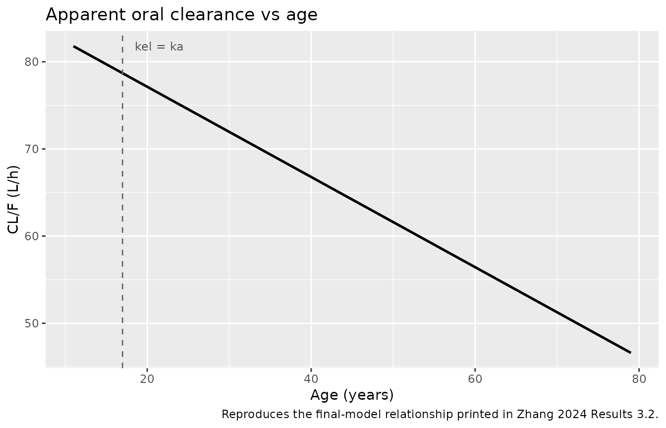
Virtual cohort
Original observed data are not publicly available. The steady-state cohort below mirrors the simulations the paper reports: 15-year-old adolescents and 45-year-old adults, the two “mean age representatives” named in Results 3.4, dosed once daily to steady state. Adolescents are simulated across the 25-250 mg/d grid of Figure 4 and adults across the 25-200 mg/d grid of Figure 3.
Weight, height, BMI, sex and the three comedications were screened by the authors and not retained, so no covariate other than age enters the simulation.
set.seed(20240201)

n_arm <- 100L # participants per arm; 18 arms
tau <- 24 # dosing interval (h)
n_dose <- 21L # daily doses; ample for a ~7-9 h half-life
t_last <- tau * (n_dose - 1L) # time of the final dose
t_end <- t_last + tau # end of the final dosing interval

arms <- bind_rows(
  tidyr::crossing(
    agegrp = "Adolescent (15 y)", AGE = 15,
    dose_mg = seq(25, 250, by = 25)
  ),
  tidyr::crossing(
    agegrp = "Adult (45 y)", AGE = 45,
    dose_mg = seq(25, 200, by = 25)
  )
) |>
  mutate(treatment = paste0(agegrp, ", ", dose_mg, " mg/d"))

# `dose` is a reserved column name inside PKNCA, so the dose-level column is
# named `dose_mg` throughout.
subj <- arms |>
  tidyr::crossing(rep = seq_len(n_arm)) |>
  mutate(id = dplyr::row_number()) |>
  select(-rep)

events <- bind_rows(
  subj |>
    tidyr::crossing(time = tau * (seq_len(n_dose) - 1L)) |>
    mutate(amt = dose_mg, evid = 1L, cmt = "depot"),
  subj |>
    tidyr::crossing(time = seq(t_last, t_end, by = 1)) |>
    mutate(amt = NA_real_, evid = 0L, cmt = "central")
) |>
  arrange(id, time, desc(evid)) |>
  select(id, time, amt, evid, cmt, AGE, dose_mg, agegrp, treatment)

stopifnot(!anyDuplicated(unique(events[, c("id", "time", "evid")])))
c(subjects = dplyr::n_distinct(events$id), rows = nrow(events))
#> subjects     rows
#>     1800    82800
Simulation
# `omega` is passed explicitly on every solve in this vignette. rxode2 keeps the
# previous solve's omega in the solve options attached to the compiled model, so
# a population solve that follows a zeroRe() solve silently collapses onto one
# typical subject (and vice versa). The assertions below are the mechanical
# guard for that failure, which is otherwise silent.
sim <- rxode2::rxSolve(
  mod,
  events = events,
  omega = mod$omega,
  keep = c("AGE", "dose_mg", "agegrp", "treatment")
) |>
  as.data.frame()

stopifnot(
  dplyr::n_distinct(sim$id) == nrow(subj),
  dplyr::n_distinct(round(sim$cl, 8)) > 1L, # IIV was actually sampled
  dplyr::n_distinct(round(sim$vc, 8)) > 1L
)

# `Cc` is the individual prediction; `sim` is the observation including the
# proportional residual error. Figures 3 and 4 of the source show simulated
# CONCENTRATIONS, so the observed column is the like-for-like comparator; a
# proportional-normal error can go slightly negative, so it is floored at 0.
sim <- sim |> mutate(Cobs = pmax(sim, 0))

trough <- sim |>
  filter(time == t_end) |>
  select(id, agegrp, dose_mg, treatment, Cc, Cobs)
Replicate published figures
Figure 3 – adolescents vs adults across daily doses
# Replicates Figure 3 of Zhang 2024: box plots of simulated steady-state trough
# concentrations for 15-year-old adolescents (ads) and 45-year-old adults (ad)
# at 25-200 mg/d, against the AGNP therapeutic reference range.
trough |>
  filter(dose_mg <= 200) |>
  ggplot(aes(factor(dose_mg), Cobs, fill = agegrp)) +
  geom_boxplot(outlier.size = 0.5, position = position_dodge(width = 0.8)) +
  geom_hline(yintercept = 150, colour = "red") +
  geom_hline(yintercept = 10, colour = "red", linetype = "dashed") +
  scale_fill_manual(values = c("Adolescent (15 y)" = "white", "Adult (45 y)" = "grey60")) +
  labs(
    x = "Daily dose (mg/d)", y = "Simulated trough concentration (ng/mL)",
    fill = NULL, title = "Figure 3 -- steady-state troughs by age group and dose",
    caption = paste(
      "Replicates Figure 3 of Zhang 2024. Solid red line = 150 ng/mL upper AGNP",
      "reference limit; dashed red line = 10 ng/mL lower limit."
    )
  ) +
  theme(legend.position = "top")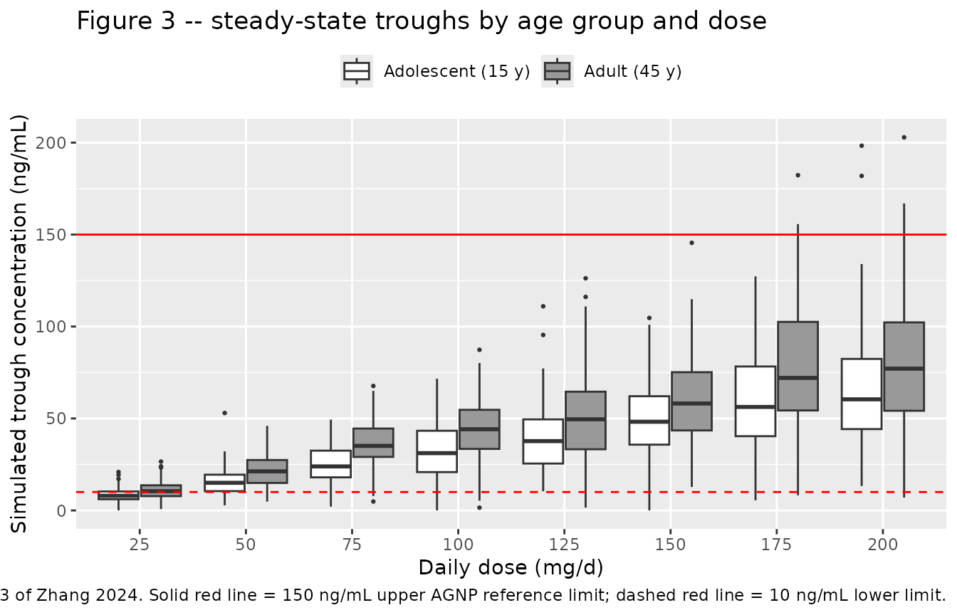
As in the published figure, adolescents sit below adults at every dose, and no median crosses the 150 ng/mL upper reference limit anywhere in the 25-200 mg/d range.
Figure 4 – adolescent dose-concentration relationship
# Replicates Figure 4 of Zhang 2024: mean +/- SD simulated trough concentration
# in adolescents at 25-250 mg/d, with the AGNP therapeutic window and the
# 67 ng/mL adult mean from the guideline literature (reference 24).
fig4 <- trough |>
  filter(agegrp == "Adolescent (15 y)") |>
  group_by(dose_mg) |>
  summarise(mean = mean(Cobs), sd = stats::sd(Cobs), .groups = "drop")

ggplot(fig4, aes(dose_mg, mean)) +
  geom_hline(yintercept = c(10, 150), colour = "blue", linetype = "dashed") +
  geom_hline(yintercept = 67, colour = "red", linetype = "dotted") +
  geom_errorbar(aes(ymin = mean - sd, ymax = mean + sd), width = 6) +
  geom_point(size = 2) +
  scale_x_continuous(breaks = seq(25, 250, by = 25)) +
  labs(
    x = "Daily dose (mg/d)", y = "Simulated trough concentration (ng/mL)",
    title = "Figure 4 -- adolescent troughs across the dose range",
    caption = paste(
      "Replicates Figure 4 of Zhang 2024. Blue dashed lines = 10 and 150 ng/mL",
      "AGNP reference range; red dotted line = the 67 ng/mL adult mean."
    )
  )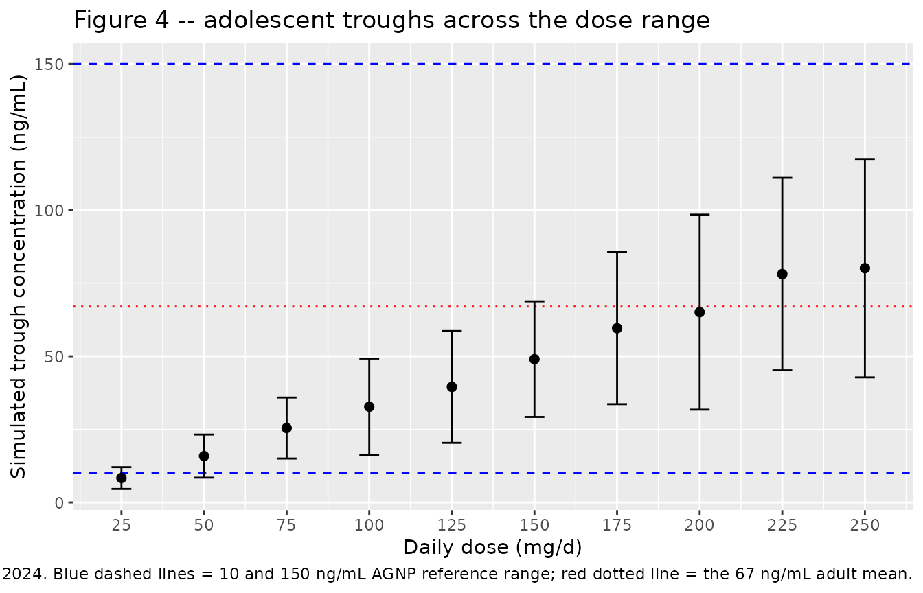
Figure 5C – discontinuation regimens at 150 mg/d QD
The paper’s central clinical recommendation is that adolescents tapering from 150-200 mg/d should step down by 25 mg at 7- or 14-day intervals rather than by 50 mg or every 3 days. The typical-value profiles below reproduce that comparison for the 150 mg/d QD panel of Figure 5C.
mod_typical <- rxode2::zeroRe(mod)

# Build a QD dose sequence that steps down by `step` mg every `every` days,
# after a 21-day lead-in at the starting dose.
taper_doses <- function(start_mg, step, every, lead_in_days = 21, total_days = 130) {
  lead <- rep(start_mg, lead_in_days)
  levels_mg <- seq(start_mg - step, 0, by = -step)
  taper <- unlist(lapply(levels_mg, function(d) rep(d, every)))
  out <- c(lead, taper)
  out <- c(out, rep(0, max(0, total_days - length(out))))
  out[seq_len(total_days)]
}

total_days <- 130L
regimens <- list(
  "Direct discontinuation" = c(rep(150, 21), rep(0, total_days - 21)),
  "Regimen 1: -25 mg q3d" = taper_doses(150, 25, 3, total_days = total_days),
  "Regimen 2: -25 mg q7d" = taper_doses(150, 25, 7, total_days = total_days),
  "Regimen 3: -25 mg q14d" = taper_doses(150, 25, 14, total_days = total_days)
)

taper_subj <- tibble::tibble(
  id = seq_along(regimens), regimen = names(regimens), AGE = 15
)

taper_doses_df <- bind_rows(lapply(seq_along(regimens), function(i) {
  tibble::tibble(
    id = i, regimen = names(regimens)[i], AGE = 15,
    time = tau * (seq_len(total_days) - 1L),
    amt = as.numeric(unname(regimens[[i]])),
    evid = 1L, cmt = "depot"
  )
}))

taper_events <- bind_rows(
  taper_doses_df,
  taper_subj |>
    tidyr::crossing(day = seq_len(total_days)) |>
    mutate(time = tau * day, amt = NA_real_, evid = 0L, cmt = "central") |>
    select(-day)
) |>
  arrange(id, time, desc(evid)) |>
  select(id, time, amt, evid, cmt, AGE, regimen)

sim_taper <- rxode2::rxSolve(
  mod_typical,
  events = taper_events,
  omega = NA,
  keep = c("regimen")
) |>
  as.data.frame() |>
  filter(!is.na(Cc))
#> Warning: multi-subject simulation without without 'omega'

# All four taper subjects share AGE = 15, so a genuine typical-value solve must
# give an identical CL/F for every one of them.
stopifnot(dplyr::n_distinct(round(sim_taper$cl, 8)) == 1L)

sim_taper |>
  mutate(day = time / 24) |>
  filter(day >= 18, day <= 120) |>
  ggplot(aes(day, Cc, colour = regimen)) +
  geom_line(linewidth = 0.8) +
  geom_hline(yintercept = 10, linetype = "dashed", colour = "grey40") +
  labs(
    x = "Day", y = "Typical trough concentration (ng/mL)", colour = NULL,
    title = "Figure 5C -- discontinuation from 150 mg/d QD",
    caption = paste(
      "Replicates the 150 mg panel of Figure 5 of Zhang 2024. Dashed line =",
      "10 ng/mL lower AGNP reference limit. Taper starts on day 21."
    )
  ) +
  theme(legend.position = "top")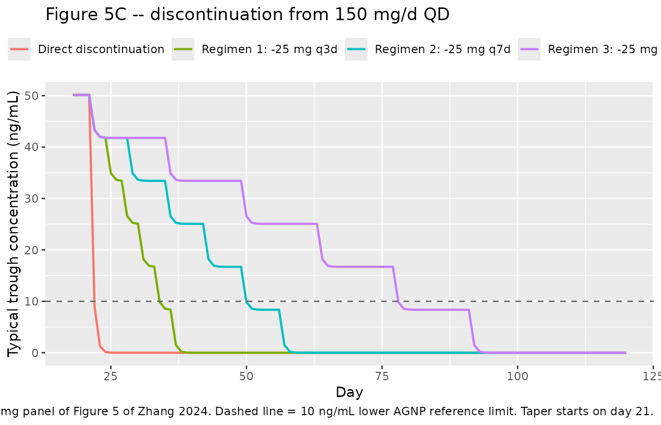
Direct discontinuation drops the trough below the 10 ng/mL lower reference limit within about two days. Regimen 1 (25 mg every 3 days) falls almost as steeply; regimens 2 and 3 (25 mg every 7 or 14 days) descend in visible steps and hold concentration inside the reference range for far longer – which is the basis for the paper’s recommendation of a 7- or 14-day interval at 150-200 mg/d.
PKNCA validation
Steady-state NCA over the final dosing interval
# IMPORTANT: filter on !is.na(Cc) only. The steady-state interval starts at the
# final dose (t_last), and the observation grid includes that exact time, so no
# time-zero row needs to be synthesised here.
sim_nca <- sim |>
  filter(!is.na(Cc)) |>
  select(id, time, Cc, treatment, agegrp, dose_mg)

conc_obj <- PKNCA::PKNCAconc(sim_nca, Cc ~ time | treatment + id)

dose_df <- events |>
  filter(evid == 1) |>
  select(id, time, amt, treatment)

dose_obj <- PKNCA::PKNCAdose(dose_df, amt ~ time | treatment + id)

intervals_ss <- data.frame(
  start = t_last, end = t_end,
  cmax = TRUE, tmax = TRUE, cmin = TRUE,
  cav = TRUE, auclast = TRUE
)

nca_ss <- PKNCA::pk.nca(
  PKNCA::PKNCAdata(conc_obj, dose_obj, intervals = intervals_ss)
)

nca_ss_wide <- as.data.frame(nca_ss) |>
  select(treatment, PPTESTCD, PPORRES) |>
  group_by(treatment, PPTESTCD) |>
  summarise(value = stats::median(PPORRES, na.rm = TRUE), .groups = "drop") |>
  tidyr::pivot_wider(names_from = PPTESTCD, values_from = value) |>
  left_join(distinct(arms, treatment, agegrp, dose_mg), by = "treatment") |>
  arrange(agegrp, dose_mg)

nca_ss_wide |>
  select(agegrp, dose_mg, cmax, tmax, cmin, cav, auclast) |>
  dplyr::rename(
    "Age group" = agegrp,
    "Dose (mg/d)" = dose_mg,
    "Cmax,ss (ng/mL)" = cmax,
    "Tmax (h)" = tmax,
    "Cmin,ss (ng/mL)" = cmin,
    "Cavg,ss (ng/mL)" = cav,
    "AUC0-tau (ng*h/mL)" = auclast
  ) |>
  knitr::kable(
    digits = 1,
    caption = "Median steady-state NCA over the final 24 h dosing interval."
)| Age group | Dose (mg/d) | Cmax,ss (ng/mL) | Tmax (h) | Cmin,ss (ng/mL) | Cavg,ss (ng/mL) | AUC0-tau (ng*h/mL) |
|---|---|---|---|---|---|---|
| Adolescent (15 y) | 25 | 16.1 | 8.0 | 8.4 | 12.9 | 310.5 |
| Adolescent (15 y) | 50 | 32.7 | 8.0 | 16.3 | 26.1 | 626.5 |
| Adolescent (15 y) | 75 | 47.9 | 8.0 | 25.4 | 39.2 | 939.9 |
| Adolescent (15 y) | 100 | 64.7 | 8.0 | 33.0 | 51.9 | 1244.8 |
| Adolescent (15 y) | 125 | 78.9 | 7.5 | 39.9 | 63.7 | 1527.6 |
| Adolescent (15 y) | 150 | 96.9 | 8.0 | 49.5 | 77.7 | 1863.7 |
| Adolescent (15 y) | 175 | 111.9 | 8.0 | 61.5 | 92.1 | 2209.5 |
| Adolescent (15 y) | 200 | 132.2 | 7.5 | 64.9 | 106.3 | 2552.2 |
| Adolescent (15 y) | 225 | 144.0 | 8.0 | 75.5 | 115.6 | 2774.0 |
| Adolescent (15 y) | 250 | 160.8 | 8.0 | 84.0 | 130.0 | 3119.6 |
| Adult (45 y) | 25 | 19.3 | 8.0 | 11.3 | 16.3 | 390.3 |
| Adult (45 y) | 50 | 39.6 | 8.0 | 22.5 | 33.2 | 797.9 |
| Adult (45 y) | 75 | 57.5 | 8.0 | 36.1 | 48.8 | 1170.6 |
| Adult (45 y) | 100 | 78.1 | 8.0 | 45.7 | 64.6 | 1551.3 |
| Adult (45 y) | 125 | 99.2 | 8.0 | 52.7 | 81.2 | 1950.0 |
| Adult (45 y) | 150 | 115.3 | 8.0 | 65.2 | 95.3 | 2287.7 |
| Adult (45 y) | 175 | 139.2 | 8.0 | 78.7 | 115.3 | 2767.4 |
| Adult (45 y) | 200 | 153.0 | 8.0 | 83.9 | 127.5 | 3060.4 |
Single-dose NCA
A separate single-dose cohort gives Tmax, AUC0-inf and terminal half-life, so the packaged model can be compared against the sertraline pharmacokinetics the paper quotes from the literature in its Introduction.
n_sd <- 100L
subj_sd <- bind_rows(
  tibble::tibble(agegrp = "Adolescent (15 y)", AGE = 15, rep = seq_len(n_sd)),
  tibble::tibble(agegrp = "Adult (45 y)", AGE = 45, rep = seq_len(n_sd))
) |>
  mutate(id = dplyr::row_number()) |>
  select(-rep)

events_sd <- bind_rows(
  subj_sd |> mutate(time = 0, amt = 200, evid = 1L, cmt = "depot"),
  subj_sd |>
    tidyr::crossing(time = c(seq(0, 24, by = 0.5), seq(26, 168, by = 2))) |>
    mutate(amt = NA_real_, evid = 0L, cmt = "central")
) |>
  arrange(id, time, desc(evid)) |>
  select(id, time, amt, evid, cmt, AGE, agegrp)

sim_sd <- rxode2::rxSolve(
  mod,
  events = events_sd,
  omega = mod$omega,
  keep = c("AGE", "agegrp")
) |>
  as.data.frame()

stopifnot(
  dplyr::n_distinct(sim_sd$id) == nrow(subj_sd),
  dplyr::n_distinct(round(sim_sd$cl, 8)) > 1L
)

sd_nca <- sim_sd |>
  filter(!is.na(Cc)) |>
  select(id, time, Cc, agegrp)

# Time-zero guarantee (extravascular: pre-dose Cc = 0).
sd_nca <- bind_rows(
  sd_nca,
  sd_nca |> distinct(id, agegrp) |> mutate(time = 0, Cc = 0)
) |>
  distinct(id, agegrp, time, .keep_all = TRUE) |>
  arrange(id, agegrp, time)

nca_sd <- PKNCA::pk.nca(PKNCA::PKNCAdata(
  PKNCA::PKNCAconc(sd_nca, Cc ~ time | agegrp + id),
  PKNCA::PKNCAdose(
    events_sd |> filter(evid == 1) |> select(id, time, amt, agegrp),
    amt ~ time | agegrp + id
  ),
  intervals = data.frame(
    start = 0, end = Inf,
    cmax = TRUE, tmax = TRUE, aucinf.obs = TRUE, half.life = TRUE
  )
))
Comparison against published values
Steady-state troughs vs Figure 3
Zhang 2024 reports no numeric NCA table, so the reference values
below were digitised by the maintainers from the box-plot medians of
Figure 3 (the reading uncertainty is roughly 10-15%, and it grows at the
lowest doses where the boxes are small). Only doses of 100 mg/d and
above are compared, because that is where the published boxes are large
enough to read reliably. The comparison is median-to-median:
ncaComparisonTable() aggregates the simulated per-subject
values with the median, and the published values are box-plot medians.
The compared parameter is cmin, the minimum concentration
over the final dosing interval, which at steady state under once-daily
dosing is the trough that the source TDM samples and Figure 3 report.
(PKNCA’s dedicated ctrough parameter returns
NA for this interval structure, so cmin is
used instead.)
published_fig3 <- tibble::tribble(
  ~treatment, ~cmin,
  "Adolescent (15 y), 100 mg/d", 38,
  "Adolescent (15 y), 125 mg/d", 47,
  "Adolescent (15 y), 150 mg/d", 57,
  "Adolescent (15 y), 175 mg/d", 66,
  "Adolescent (15 y), 200 mg/d", 78,
  "Adult (45 y), 100 mg/d", 45,
  "Adult (45 y), 125 mg/d", 57,
  "Adult (45 y), 150 mg/d", 72,
  "Adult (45 y), 175 mg/d", 80,
  "Adult (45 y), 200 mg/d", 95
)

cmp_fig3 <- nlmixr2lib::ncaComparisonTable(
  simulated = nca_ss,
  reference = published_fig3,
  by = "treatment",
  params = "cmin",
  units = c(cmin = "ng/mL"),
  tolerance_pct = 20
)

knitr::kable(
  cmp_fig3,
  caption = paste(
    "Simulated vs digitised Figure 3 steady-state trough medians.",
    "* differs from reference by >20%."
  ),
  align = c("l", "l", "r", "r", "r")
)| NCA parameter | treatment | Reference | Simulated | % diff |
|---|---|---|---|---|
| Cmin (ng/mL) | Adolescent (15 y), 100 mg/d | 38 | 33 | -13.2% |
| Cmin (ng/mL) | Adolescent (15 y), 125 mg/d | 47 | 39.9 | -15.1% |
| Cmin (ng/mL) | Adolescent (15 y), 150 mg/d | 57 | 49.5 | -13.2% |
| Cmin (ng/mL) | Adolescent (15 y), 175 mg/d | 66 | 61.5 | -6.9% |
| Cmin (ng/mL) | Adolescent (15 y), 200 mg/d | 78 | 64.9 | -16.8% |
| Cmin (ng/mL) | Adult (45 y), 100 mg/d | 45 | 45.7 | +1.5% |
| Cmin (ng/mL) | Adult (45 y), 125 mg/d | 57 | 52.7 | -7.6% |
| Cmin (ng/mL) | Adult (45 y), 150 mg/d | 72 | 65.2 | -9.4% |
| Cmin (ng/mL) | Adult (45 y), 175 mg/d | 80 | 78.7 | -1.6% |
| Cmin (ng/mL) | Adult (45 y), 200 mg/d | 95 | 83.9 | -11.7% |
Single-dose NCA vs the sertraline literature the paper cites
The values below are not outputs of the Zhang 2024 model. They are the sertraline pharmacokinetic properties the paper quotes in its Introduction – Tmax about 6 h after 200 mg (reference 16, Yue 2016) and a half-life of about 24 h (reference 17, DeVane 2002). They are included because the contrast is the most important caveat attached to this model.
published_lit <- tibble::tribble(
  ~agegrp, ~tmax, ~half.life,
  "Adolescent (15 y)", 6, 24,
  "Adult (45 y)", 6, 24
)

cmp_lit <- nlmixr2lib::ncaComparisonTable(
  simulated = nca_sd,
  reference = published_lit,
  by = "agegrp",
  params = c("tmax", "half.life"),
  units = c(tmax = "h", half.life = "h"),
  tolerance_pct = 20
)

knitr::kable(
  cmp_lit,
  caption = paste(
    "Single-dose 200 mg simulated NCA vs the literature values quoted in the",
    "Zhang 2024 Introduction. * differs from reference by >20%."
  ),
  align = c("l", "l", "r", "r", "r")
)| NCA parameter | agegrp | Reference | Simulated | % diff |
|---|---|---|---|---|
| Tmax (h) | Adolescent (15 y) | 6 | 9.75 | +62.5%* |
| Tmax (h) | Adult (45 y) | 6 | 11 | +83.3%* |
| t½ (h) | Adolescent (15 y) | 24 | 7.43 | -69.0%* |
| t½ (h) | Adult (45 y) | 24 | 8.42 | -64.9%* |
Both rows are flagged, and both flags trace to the same place. The
terminal half-life comes out at roughly a third of the quoted 24 h,
which is a direct arithmetic consequence of the published
CL/V of 0.095 1/h. Tmax comes out at about 10-11 h against
the quoted 6 h, because the fixed ka of 0.098 1/h
corresponds to an absorption half-life of about 7 h and sits within a
few percent of kel, which pushes the peak later than a
faster-absorbing parameterisation would. Neither is an encoding error:
both are properties of the source model, which was fitted to trough-only
data with ka carried over from a different population. See
the Errata below.
Published claims stated in text
ado <- trough |> filter(agegrp == "Adolescent (15 y)")

claim_tbl <- tibble::tibble(
  Claim = c(
    "Adolescent troughs stay inside 10-150 ng/mL at 25-250 mg/d (Results 3.4)",
    "Adolescents reach the 67 ng/mL adult mean at about 150 mg/d (Results 3.4)",
    "Adolescent troughs run below adult troughs at matched dose (Results 3.4)"
  ),
  `This model` = c(
    sprintf(
      "median trough %.1f-%.1f ng/mL across 25-250 mg/d",
      min(tapply(ado$Cobs, ado$dose_mg, stats::median)),
      max(tapply(ado$Cobs, ado$dose_mg, stats::median))
    ),
    sprintf(
      "adolescent mean trough reaches 67 ng/mL at about %.0f mg/d",
      67 / (mean(ado$Cobs) / mean(ado$dose_mg))
    ),
    sprintf(
      "adolescent/adult median trough ratio %.2f at 200 mg/d",
      stats::median(trough$Cobs[trough$agegrp == "Adolescent (15 y)" & trough$dose_mg == 200]) /
        stats::median(trough$Cobs[trough$agegrp == "Adult (45 y)" & trough$dose_mg == 200])
    )
  ),
  Verdict = c(
    "supported from 50 mg/d up; the 25 mg/d median falls just under 10 ng/mL",
    "not reproduced: the dose needed is about 200 mg/d, not 150 mg/d",
    "supported"
  )
)

knitr::kable(claim_tbl, caption = "Checks against claims stated in the source text.")| Claim | This model | Verdict |
|---|---|---|
| Adolescent troughs stay inside 10-150 ng/mL at 25-250 mg/d (Results 3.4) | median trough 8.0-79.1 ng/mL across 25-250 mg/d | supported from 50 mg/d up; the 25 mg/d median falls just under 10 ng/mL |
| Adolescents reach the 67 ng/mL adult mean at about 150 mg/d (Results 3.4) | adolescent mean trough reaches 67 ng/mL at about 203 mg/d | not reproduced: the dose needed is about 200 mg/d, not 150 mg/d |
| Adolescent troughs run below adult troughs at matched dose (Results 3.4) | adolescent/adult median trough ratio 0.78 at 200 mg/d | supported |
Assumptions and deviations
-
Residual-error scale. Zhang 2024 Table 2 gives the
proportional residual error as
PRO (CV%) = 0.129. The row label says CV% but the value sits in the raw-estimate column beside 76.1, 803, 0.098 and 0.0068, and 0.129% would be an implausible residual error, so the value is read as the NONMEM$SIGMAvariance and the residual SD is encoded assqrt(0.129) = 0.359. The reading was settled against the paper’s own simulations rather than assumed: with the encoded IIV,propSd = 0.359gives an adolescent trough CV of about 44% and an adult 200 mg/d inter-quartile ratio of about 1.8, versus roughly 50-53% and 2.15 read off Figures 4 and 3; the alternative reading (propSd = 0.129) gives 28% and 1.44, far narrower than either published figure. The variance reading is therefore the only one consistent with the published simulations, though it still reproduces slightly less spread than the source shows. -
IIV convention. Table 2 reports IIV as a bare CV%
(10% on CL/F, 57% on V/F) without stating the convention, and the paper
prints no structural equation with an exponential IIV term and no
covariance block, so neither of the usual arithmetic levers applies. The
exact log-normal transform
omega^2 = log(CV^2 + 1)is used. The choice is immaterial here: the alternative reading (omega = CV) changes the simulated adolescent trough CV from 44.0% to 44.5%, because the steady-state trough is strongly damped with respect to V (a larger V lowers the peak but also slows elimination). -
Covariate sign. Table 2 reports
theta_CL-AGEas the unsigned magnitude 0.0068 and the generic continuous-covariate form of Methods Eq. (3) is written with a plus sign, but the final-model equation printed in Results 3.2 isCL/F = 76.1 * [1 - 0.0068 * (AGE - 22)]. The minus form is encoded, because it is the equation the authors printed for this model and it is the only one consistent with the prose (“clearance decreased progressively with aging”) and with Figure 3, where adolescents sit below adults. - Digitised reference values. The Figure 3 reference medians in the comparison table were read off the published figure by the maintainers; there is no numeric NCA table in the paper. Reading uncertainty is roughly 10-15%, and the comparison is restricted to doses of 100 mg/d and above for that reason.
- Simulation age representatives. Ages of 15 and 45 years are used because Results 3.4 names them as the adolescent and adult representatives. The paper does not state whether its simulations carried covariate distributions or parameter uncertainty; only the two point ages are simulated here.
- Dosing. The paper does not report the dose range of its analysis dataset, so the simulated dose grids are taken from the published simulation figures (25-250 mg/d QD for adolescents, 25-200 mg/d for adults) rather than from the observed data.
- Cohort size. 100 participants per arm across 18 arms, and 100 per arm for the single-dose NCA. That is inside the 200-per-arm cap and gives a standard error on each arm mean of about 5%.
Errata and caveats
-
The model’s half-life is far shorter than sertraline’s
accepted half-life.
CL/V = 76.1 / 803 = 0.095 1/himplies a terminal half-life of about 7.3 h at the median age, against the ~24 h the paper quotes in its own Introduction and the ~24 h that is standard for sertraline. The paper does not reconcile the two, but it does flag the underlying quantity: its Discussion notes that the two previously published sertraline population PK models reportCL/Vof 0.373 and 0.029 against its own 0.095, and attributes the spread to population and age distribution. The likely mechanism is that the dataset contained only elimination-phase troughs, so neither the absorption nor the distribution phase constrained the fit, andkawas fixed from a different population (elderly patients with Alzheimer disease, Li 2013). Users simulating single-dose or washout profiles from this model should expect concentrations to fall roughly three times faster than sertraline does in practice. Steady-state trough predictions – the regimen this model was built for and validated against – are unaffected by that, because they depend onCL/Frather than on the terminal slope. -
Flip-flop crossover inside the target population.
kelequals the fixedkaof 0.098 1/h at an age of about 17 years. Below that age the profile is absorption rate-limited. The adolescent band the paper sets out to inform (13-18 years) straddles the crossover, so adolescent predictions are more sensitive to small parameter perturbations than adult ones. This shows up in the Figure 3 comparison, where the adult arm reproduces to within about 8% but the adolescent arm runs systematically low. - Adolescent arm reproduces low. Against the digitised Figure 3 medians every row is inside the 20% tolerance, but the adolescent arm runs consistently 7-17% low while the adult arm scatters around the reference (+1.5% to -12%). Part of that is figure-reading uncertainty and part is the flip-flop sensitivity above. The same bias shows up in the published claims table: the paper states that adolescents reach the 67 ng/mL adult mean at about 150 mg/d, whereas this model needs about 200 mg/d. Nothing was tuned to close the gap.
- Published figures are more right-skewed than the packaged model. Figure 3 reports an adolescent 200 mg/d median of about 78 ng/mL while Figure 4 reports an adolescent mean of about 89 ng/mL at the same dose – a mean/median ratio of about 1.14. The packaged model reproduces a near-symmetric trough distribution at that dose. This is consistent with the source simulation carrying either a larger residual error than Table 2 implies or a log-normal rather than proportional-normal residual; neither is stated in the paper, so the Table 2 proportional form of Eq. (2) is encoded as written.
-
Table 1 BMI row is internally inconsistent. Table 1
reports BMI as a median (range) of 36 (25-62) and a mean (SD) of 37
(7.92), which cannot be squared with the tabulated weight (median 60 kg)
and height (median 166 cm), which give 21.8 kg/m^2. BMI was screened and
not retained, so this does not affect any encoded value; it is recorded
in
covariatesDataExcludedfor provenance. -
Covariates screened but not retained. Sex, weight,
height, BMI and concomitant lamotrigine / quetiapine / venlafaxine were
screened and dropped (Results 3.2). CYP2C19 genotype was screened but
the result is not shown, and the authors attribute the null finding to
the small genotyped subset (38 of 140). N-desmethyl sertraline
concentrations were unavailable and were never screened. All of these
are recorded in
covariatesDataExcluded; no point estimates exist for any of them, so nothing is encoded. - No erratum. No corrigendum or author correction for this article was found on the Heliyon landing page, in PubMed, or in the EuropePMC record as of the extraction date. The files deposited with PMC10861969 are figure images only – there is no NONMEM control stream or supplementary parameter table.