Ustekinumab PK and clearance-response in inflammatory bowel disease (Yarur 2025)
Source:vignettes/articles/Yarur_2025_ustekinumab.Rmd
Yarur_2025_ustekinumab.Rmd
library(nlmixr2lib)
library(PKNCA)
#>
#> Attaching package: 'PKNCA'
#> The following object is masked from 'package:stats':
#>
#>     filter
library(rxode2)
#> rxode2 5.1.8 using 2 threads (see ?getRxThreads)
#>   no cache: create with `rxCreateCache()`
library(dplyr)
#>
#> Attaching package: 'dplyr'
#> The following objects are masked from 'package:stats':
#>
#>     filter, lag
#> The following objects are masked from 'package:base':
#>
#>     intersect, setdiff, setequal, union
library(tidyr)
library(ggplot2)
Model and source
Yarur 2025 contributes six models to the library: one population PK model (the “Final Bayesian Priors” column of Table 1) and five independently fitted logistic exposure-response (ER) models from Supplementary Table S1. All six share this vignette.
#> ℹ parameter labels from comments will be replaced by 'label()'Citation: Yarur AJ, Dervieux T, Ungaro R, Spencer EA, Bruss A, Nunez L, Berens B, Vermeire S, Wang Z, Panetta JC, Dreesen E, Dubinsky MC. Ustekinumab Drug Clearance Is Better Associated with Disease Control than Serum Trough Concentrations in a Prospective Cohort of Inflammatory Bowel Disease. Pharmaceutics. 2025;17(2):187. doi:10.3390/pharmaceutics17020187. Model structure from Wang Z, Verstockt B, Sabino J, Vermeire S, Ferrante M, Declerck P, Dreesen E. Br J Clin Pharmacol. 2022;88(1):323-335. doi:10.1111/bcp.14971.
Description (population PK): Two-compartment population PK model with first-order subcutaneous absorption for ustekinumab in adults and adolescents with inflammatory bowel disease, with concentrations measured by the drug-tolerant homogeneous mobility shift assay (HMSA) (Yarur 2025). This is the ‘Final Bayesian Priors’ model of Table 1: the Wang 2022 Crohn’s disease model structure re-fitted to HMSA re-assayed samples (albumin power effect on CL), plus an antibodies-to-ustekinumab (ATU) effect on CL estimated from a clinical PK-laboratory database, with between-subject variability on CL only. The paper used it, with every parameter fixed, to obtain empirical-Bayes clearances for the Yarur_2025_ustekinumab_* exposure-response models.
Article: https://doi.org/10.3390/pharmaceutics17020187 (open access)
Supplement: Table S1, “Estimates from logistic regression models”, https://www.mdpi.com/article/10.3390/pharmaceutics17020187/s1.
Upstream model structure: Wang Z et al. Br J Clin Pharmacol 2022;88(1):323-335, https://doi.org/10.1111/bcp.14971.
| Model | Endpoint | Regressors | Source |
|---|---|---|---|
Yarur_2025_ustekinumab |
serum ustekinumab (HMSA) | albumin, ATU on CL | Table 1, “Final Bayesian Priors” |
Yarur_2025_ustekinumab_clinbiorem_time |
clinical and biochemical remission | prior biologics, time | Table S1, row 1 |
Yarur_2025_ustekinumab_clinbiorem_ctrough |
clinical and biochemical remission | prior biologics, trough | Table S1, row 2; Figure 2A |
Yarur_2025_ustekinumab_clinbiorem_cl |
clinical and biochemical remission | prior biologics, clearance | Table S1, row 3; Figure 2B |
Yarur_2025_ustekinumab_ehi50_ctrough |
EHI > 50 points | prior biologics, trough | Table S1, row 4; Figure 3A |
Yarur_2025_ustekinumab_ehi50_cl |
EHI > 50 points | prior biologics, clearance | Table S1, row 5; Figure 3B |
How the paper built the PK model
Ustekinumab concentrations in this study were measured with a
drug-tolerant homogeneous mobility shift assay (HMSA), which reads about
1.5-fold higher than the solid-phase ELISA used by the earlier Wang 2022
Crohn’s disease popPK study. The authors therefore (1) re-assayed the
Wang 2022 training samples (308 concentrations, 65 patients) with the
HMSA and re-fitted the same model structure in NONMEM 7.5; (2) fixed
that fit and estimated an antibodies-to-ustekinumab (ATU) effect on
clearance from 11,372 clinical PK-laboratory specimens; and (3) fixed
every parameter as a Bayesian prior to obtain individual clearances for
the 83-patient prospective cohort in Monolix.
Yarur_2025_ustekinumab is the model of step 3.
The prospective-cohort clearances then entered mixed-effects logistic
regressions of each outcome on one PK metric (trough or clearance) or on
time, each with prior biologic exposure as a covariate:
logit(P) = theta_pop + theta_prior * PRIOR_BIO + theta_x * x.
Population
The PK model’s structural and albumin parameters come from 65 adults with Crohn’s disease in the Wang 2022 training cohort; Yarur 2025 does not reprint their demographics. The ER models were fitted to the prospective two-centre US cohort (Table 4): 83 patients (52% female, median age 42 years, IQR 28-57; 78 Crohn’s disease and 5 ulcerative colitis), all on ustekinumab maintenance for at least 16 weeks after a weight-based IV loading dose, followed over 312 dose cycles (median 3 per patient). 77 cycles were on every-4-week dosing and the rest mostly on every-8-week dosing (median inter-dose interval 56 days, IQR 42-56). Median albumin was 3.8 g/dL (IQR 3.5-4.1); 89% (74/83) had prior biologic exposure; no sample was ATU-positive.
str(pk_ui$population)
#> List of 8
#>  $ species       : chr "human"
#>  $ n_subjects    : int 65
#>  $ n_studies     : int 1
#>  $ n_observations: chr "308 HMSA re-assayed serum concentrations (training cohort); ATU effect from 11,372 PK-laboratory specimens"
#>  $ disease_state : chr "Crohn's disease (training cohort); the Bayesian application cohort had Crohn's disease (78/83) or ulcerative colitis (5/83)"
#>  $ dose_range    : chr "IV weight-based loading dose then 90 mg SC every 8 weeks (training cohort); 90 mg SC every 4-8 weeks maintenanc"| __truncated__
#>  $ regions       : chr "Belgium (training cohort, Wang 2022); United States (application cohort and PK-laboratory database)"
#>  $ notes         : chr "The structural and albumin parameters were estimated on 308 samples from 65 Crohn's disease patients of the Wan"| __truncated__
Source trace
Every ini() entry carries an in-file comment naming its
source. The table collects them.
| Model / parameter | Value | Source location |
|---|---|---|
PK lka
|
log(0.142) fixed, 1/day |
Table 1, Ka (all columns) |
PK lfdepot
|
log(0.735) fixed |
Table 1, Bioavailability, Final Bayesian Priors |
PK lcl
|
log(0.161) fixed, L/day |
Table 1, CL_pop |
PK lvc
|
log(3.72) fixed, L |
Table 1, V1_pop |
PK lq
|
log(0.0322) fixed, L/day |
Table 1, Q |
PK lvp
|
log(0.393) fixed, L |
Table 1, V2 |
PK e_ada_cl
|
0.566 fixed | Table 1, effect of ATU on CL; footnote covariate model 1 |
PK e_alb_cl
|
-0.887 fixed | Table 1, effect of ALB on CL; footnote covariate model 2 |
PK etalcl
|
variance 0.0924 (30.4%) fixed | Table 1, IIV of CL |
PK propSd
|
0.11 fixed | Table 1, Proportional error 11.0% |
PK addSd
|
0.495 ug/mL fixed | Table 1, Additive error |
PK cl equation |
CLpop * (ALB_gdL / 4.0)^beta_ALB * exp(beta_ATU * ATU) |
Table 1 footnote |
| PK structure | 2-compartment, first-order SC absorption with F | Methods 2.3, Table 1 |
| clinbiorem_time | 0.006, -2.48, +0.0024 /day | Table S1 row 1 |
| clinbiorem_ctrough | 0.22, -2.36, +0.024 per ug/mL | Table S1 row 2 |
| clinbiorem_cl | 2.29, -2.02, -13.5 per L/day | Table S1 row 3 |
| ehi50_ctrough | -1.85, -0.52, -0.072 per ug/mL | Table S1 row 4 |
| ehi50_cl | -6.29, +0.639, +18.0 per L/day | Table S1 row 5 |
| logistic link | logit(P) = theta_pop + cov1*theta_cov1 + cov2*theta_cov2 |
Table S1 footnote |
Population PK simulation
Virtual cohort
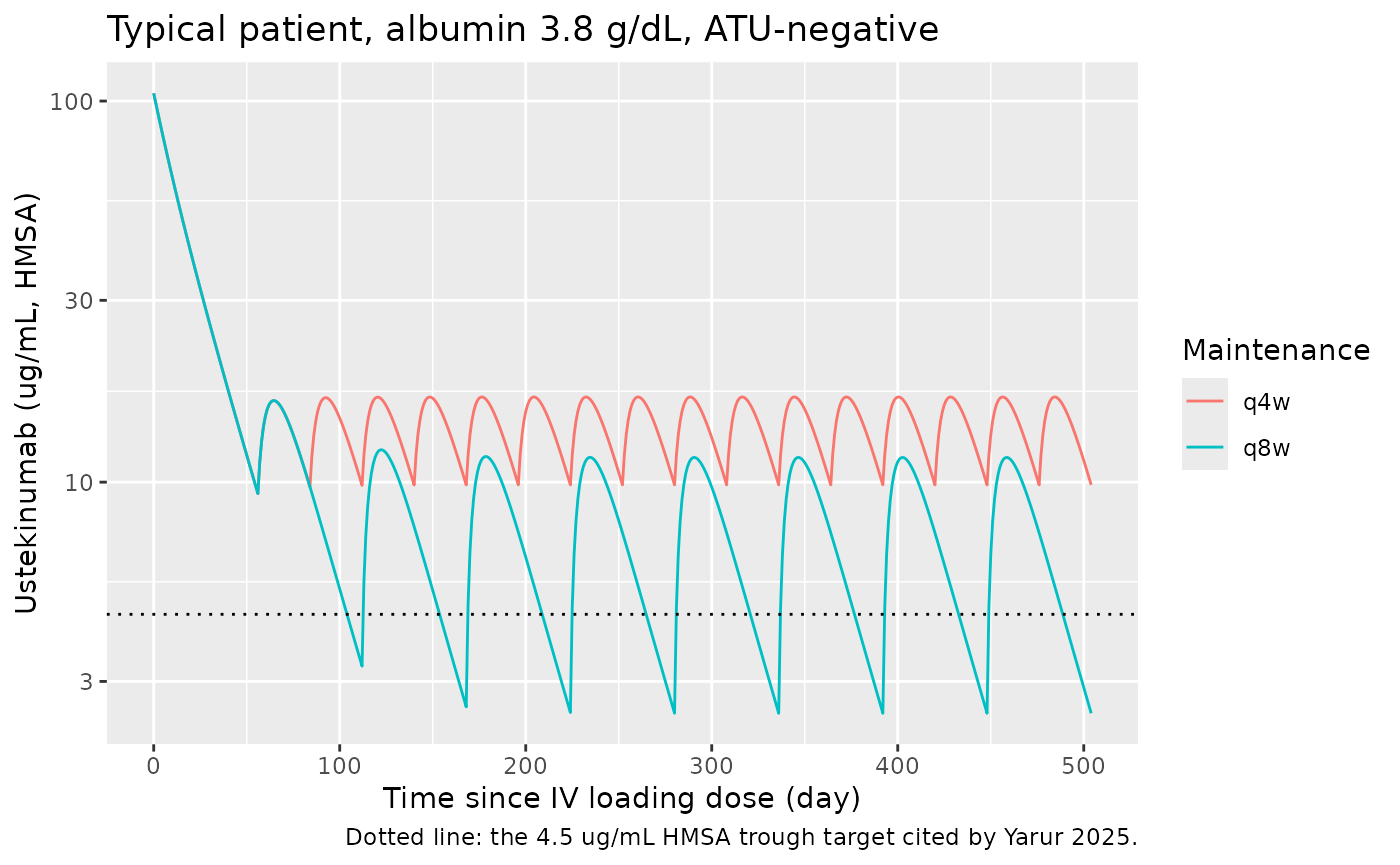
The cohort mimics the prospective maintenance population: an IV loading dose of 390 mg (the label dose for 55-85 kg) on day 0, then 90 mg SC from week 8 every 8 weeks or, in a quarter of the patients (matching 77 of 312 cycles), every 4 weeks. Albumin is drawn from a normal distribution matching the Table 4 median and IQR (3.8 g/dL; IQR 3.5-4.1, so SD about 0.44 g/dL) and held constant; everyone is ATU-negative, as in the study.
set.seed(20251025)
rxode2::rxSetSeed(20251025)

n_q8w <- 150L
n_q4w <- 50L
t_end <- 504

make_arm <- function(n, regimen, tau, id_offset) {
  alb_gdl <- pmin(pmax(rnorm(n, 3.8, 0.44), 2.5), 5.0)
  subj <- tibble(
    id = id_offset + seq_len(n),
    regimen = regimen,
    ALB = 10 * alb_gdl,
    ADA_POS = 0L
  )
  sc_times <- seq(56, t_end - tau, by = tau)
  doses <- bind_rows(
    tibble(time = 0, amt = 390, cmt = "central"),
    tibble(time = sc_times, amt = 90, cmt = "depot")
  )
  obs <- tibble(time = seq(0, t_end, by = 1), amt = 0, cmt = "central")
  tidyr::expand_grid(subj, bind_rows(
    mutate(doses, evid = 1L),
    mutate(obs, evid = 0L)
  )) |>
    arrange(id, time, desc(evid))
}

events <- bind_rows(
  make_arm(n_q8w, "q8w", 56, 0L),
  make_arm(n_q4w, "q4w", 28, n_q8w)
)
stopifnot(!anyDuplicated(events[events$evid == 1, c("id", "time")]))
Simulation
sim <- rxode2::rxSolve(
  pk_ui,
  events = events,
  keep = c("regimen", "ALB")
) |>
  as.data.frame()
Typical concentration-time profile
pk_typ <- pk_ui |> rxode2::zeroRe()
ev_typ <- events |>
  filter(id %in% c(1L, n_q8w + 1L)) |>
  mutate(ALB = 38)
sim_typ <- rxode2::rxSolve(pk_typ, events = ev_typ, keep = "regimen") |>
  as.data.frame()
#> ℹ omega/sigma items treated as zero: 'etalcl'
#> Warning: multi-subject simulation without without 'omega'

ggplot(sim_typ, aes(time, Cc, colour = regimen)) +
  geom_line() +
  geom_hline(yintercept = 4.5, linetype = "dotted") +
  scale_y_log10() +
  labs(
    x = "Time since IV loading dose (day)",
    y = "Ustekinumab (ug/mL, HMSA)",
    colour = "Maintenance",
    title = "Typical patient, albumin 3.8 g/dL, ATU-negative",
    caption = "Dotted line: the 4.5 ug/mL HMSA trough target cited by Yarur 2025."
  )
Steady-state troughs and clearance against Table 4
Table 4 reports the observed troughs and the Bayesian clearances over all 312 cycles. The simulated troughs are the pre-dose concentrations of the last maintenance interval, pooled with the same 1:3 mix of every-4-week and every-8-week dosing.
troughs <- sim |>
  filter(time == t_end) |>
  select(id, regimen, Ctrough = Cc, cl)

trough_summary <- troughs |>
  summarise(
    `Median Ctrough (ug/mL)` = median(Ctrough),
    `Q1 Ctrough` = quantile(Ctrough, 0.25),
    `Q3 Ctrough` = quantile(Ctrough, 0.75),
    `Median CL (L/day)` = median(cl),
    `Q1 CL` = quantile(cl, 0.25),
    `Q3 CL` = quantile(cl, 0.75)
  ) |>
  mutate(Source = "Simulated (pooled 1:3 q4w:q8w)")

published_t4 <- tibble(
  Source = "Observed, Yarur 2025 Table 4",
  `Median Ctrough (ug/mL)` = 5.0, `Q1 Ctrough` = 3.0, `Q3 Ctrough` = 8.7,
  `Median CL (L/day)` = 0.157, `Q1 CL` = 0.120, `Q3 CL` = 0.190
)

bind_rows(published_t4, trough_summary) |>
  relocate(Source) |>
knitr::kable(digits = 3, caption = "Trough concentrations and clearance: simulated vs. Table 4.")| Source | Median Ctrough (ug/mL) | Q1 Ctrough | Q3 Ctrough | Median CL (L/day) | Q1 CL | Q3 CL |
|---|---|---|---|---|---|---|
| Observed, Yarur 2025 Table 4 | 5.000 | 3.000 | 8.700 | 0.157 | 0.120 | 0.190 |
| Simulated (pooled 1:3 q4w:q8w) | 3.215 | 2.006 | 6.275 | 0.169 | 0.139 | 0.211 |
troughs |>
  group_by(regimen) |>
  summarise(
    `Median Ctrough (ug/mL)` = median(Ctrough),
    `% above 4.5 ug/mL` = 100 * mean(Ctrough > 4.5),
    .groups = "drop"
  ) |>
knitr::kable(digits = 2, caption = "Simulated steady-state troughs by maintenance interval.")| regimen | Median Ctrough (ug/mL) | % above 4.5 ug/mL |
|---|---|---|
| q4w | 8.34 | 96.00 |
| q8w | 2.63 | 19.33 |
The simulated clearance matches the cohort’s Bayesian clearances closely; its spread is wider, as expected, because the observed values are empirical-Bayes estimates from one trough per cycle and shrink towards the typical value.
The simulated troughs are lower than the observed ones (a typical every-8-week patient with albumin 3.8 g/dL reaches about 2.5 ug/mL). This is a property of the published model applied to this cohort, not of the transcription: the cohort’s median Bayesian clearance (0.157 L/day) is already below the typical value the prior predicts at the cohort’s median albumin (0.161 x (3.8/4.0)^-0.887 = 0.169 L/day), i.e. the measured troughs pulled the individual clearances down, and empirical-Bayes shrinkage limits how far. The dosing mix is also only approximated: Table 4 gives an inter-dose interval IQR of 42-56 days, so some cycles were on 6-week dosing, which the 1:3 mix ignores.
pooled_med <- median(troughs$Ctrough)
cl_med <- median(troughs$cl)
stopifnot(
  # Clearance: tests CL_pop and the albumin exponent directly against the
  # cohort's Bayesian estimates.
  abs(cl_med / 0.157 - 1) < 0.15,
  # Trough: only a coarse guard against unit or bioavailability errors
  # (a mg-vs-ug or F slip moves it several-fold); see the text for why the
  # model sits below the observed median.
  pooled_med > 0.4 * 5.0,
  pooled_med < 1.2 * 5.0
)
Covariate effects
cl_rel <- tibble(
  ALB_gdL = c(3.0, 3.5, 4.0, 4.5)
) |>
  mutate(
    `CL (L/day), ATU-negative` = 0.161 * (ALB_gdL / 4.0)^-0.887,
    `CL (L/day), ATU-positive` = `CL (L/day), ATU-negative` * exp(0.566)
  )
knitr::kable(cl_rel, digits = 3, caption = "Typical clearance by albumin and ATU status (Table 1 footnote).")| ALB_gdL | CL (L/day), ATU-negative | CL (L/day), ATU-positive |
|---|---|---|
| 3.0 | 0.208 | 0.366 |
| 3.5 | 0.181 | 0.319 |
| 4.0 | 0.161 | 0.284 |
| 4.5 | 0.145 | 0.255 |
PKNCA validation
The paper reports no NCA beyond the trough, so PKNCA is run on the last steady-state dosing interval of each regimen and the pooled minimum concentration is compared with the Table 4 median trough.
sim_nca <- sim |>
  filter(!is.na(Cc)) |>
  select(id, time, Cc, regimen)

dose_df <- events |>
  filter(evid == 1) |>
  select(id, time, amt, regimen)

conc_obj <- PKNCA::PKNCAconc(sim_nca, Cc ~ time | regimen + id)
dose_obj <- PKNCA::PKNCAdose(dose_df, amt ~ time | regimen + id)

intervals <- data.frame(
  regimen = c("q8w", "q4w"),
  start = c(t_end - 56, t_end - 28),
  end = c(t_end, t_end),
  cmax = TRUE,
  tmax = TRUE,
  cmin = TRUE,
  cav = TRUE
)
nca_res <- PKNCA::pk.nca(PKNCA::PKNCAdata(conc_obj, dose_obj, intervals = intervals))

nca_res$result |>
  filter(PPTESTCD %in% c("cmax", "tmax", "cmin", "cav")) |>
  group_by(regimen, PPTESTCD) |>
  summarise(median = median(PPORRES), .groups = "drop") |>
  tidyr::pivot_wider(names_from = PPTESTCD, values_from = median) |>
  rename(
    "Regimen" = regimen,
    "Cmax (ug/mL)" = cmax,
    "Tmax (day)" = tmax,
    "Cmin (ug/mL)" = cmin,
    "Cav (ug/mL)" = cav
  ) |>
knitr::kable(digits = 2, caption = "Simulated steady-state NCA (median per regimen).")| Regimen | Cav (ug/mL) | Cmax (ug/mL) | Cmin (ug/mL) | Tmax (day) |
|---|---|---|---|---|
| q4w | 12.45 | 15.17 | 8.34 | 8 |
| q8w | 7.21 | 11.81 | 2.63 | 11 |
sim_pooled <- nca_res$result |>
  filter(PPTESTCD == "cmin") |>
  mutate(group = "All cycles (1:3 q4w:q8w)") |>
  select(group, PPTESTCD, PPORRES)

published_nca <- tibble(group = "All cycles (1:3 q4w:q8w)", cmin = 5.0)

cmp <- nlmixr2lib::ncaComparisonTable(
  simulated = sim_pooled,
  reference = published_nca,
  by = "group",
  units = c(cmin = "ug/mL"),
  tolerance_pct = 20
)
knitr::kable(cmp, caption = "Simulated steady-state Cmin vs. the Table 4 median trough. * differs by >20%.")| NCA parameter | group | Reference | Simulated | % diff |
|---|---|---|---|---|
| Cmin (ug/mL) | All cycles (1:3 q4w:q8w) | 5 | 3.21 | -35.7%* |
The Cmin row is expected to be flagged: as explained above, the model under-predicts this cohort’s observed troughs, and the cohort’s own Bayesian clearances show the same shift. No parameter was adjusted.
Exposure-response models
er_names <- c(
  "Yarur_2025_ustekinumab_clinbiorem_time",
  "Yarur_2025_ustekinumab_clinbiorem_ctrough",
  "Yarur_2025_ustekinumab_clinbiorem_cl",
  "Yarur_2025_ustekinumab_ehi50_ctrough",
  "Yarur_2025_ustekinumab_ehi50_cl"
)
er_mods <- lapply(er_names, function(n) rxode2::rxode(readModelDb(n)))
names(er_mods) <- sub("^Yarur_2025_ustekinumab_", "", er_names)

# One subject per grid row (rxSolve drops the id column for single-subject
# solves); observations at a single time.
er_solve <- function(key, grid, time = 0) {
  ev <- grid |>
    mutate(id = row_number(), time = time, amt = 0, evid = 0L)
  out <- paste0("prob_", sub("_.*", "", key))
  s <- as.data.frame(rxode2::rxSolve(er_mods[[key]], events = ev))
  stopifnot(nrow(s) == nrow(grid))
  grid[[out]] <- s[[out]][order(s$id)]
  grid
}
prior_lab <- function(x) ifelse(x == 1, "experienced", "naive")
Remission at the median follow-up (Results 3.3)
time_chk <- er_solve(
  "clinbiorem_time",
  tibble(PRIOR_BIO = c(0L, 1L)),
  time = 279
) |>
  mutate(Published = c(0.66, 0.14), `Prior biologics` = prior_lab(PRIOR_BIO))
#> Warning: multi-subject simulation without without 'omega'
time_chk |>
  select(`Prior biologics`, Model = prob_clinbiorem, Published) |>
knitr::kable(digits = 3, caption = "Probability of clinical and biochemical remission at 279 days (Results 3.3).")| Prior biologics | Model | Published |
|---|---|---|
| naive | 0.663 | 0.66 |
| experienced | 0.141 | 0.14 |
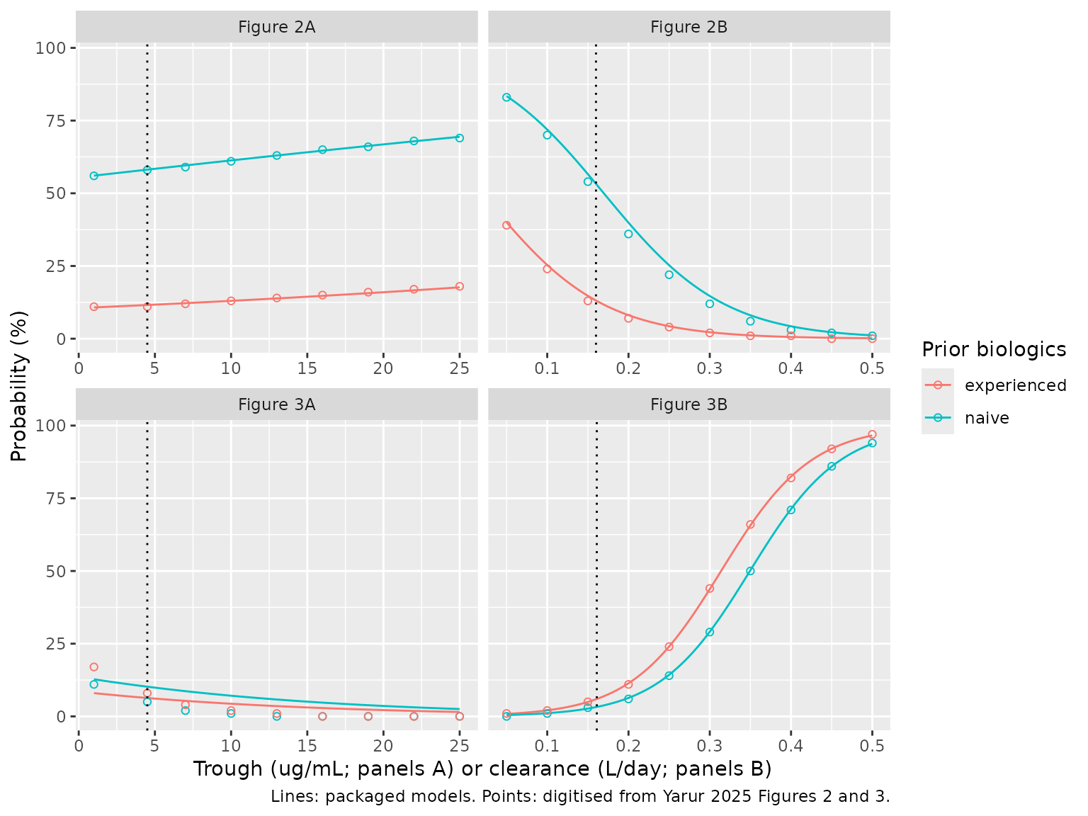
Figures 2 and 3
The published curves were digitised by the maintainers (read-off precision about 2 percentage points) and overlaid as points on the model curves.
x_conc <- c(1, 4.5, 7, 10, 13, 16, 19, 22, 25)
x_cl <- seq(0.05, 0.5, by = 0.05)
digitised <- bind_rows(
  tibble(panel = "Figure 2A", x = x_conc, PRIOR_BIO = 0L, pct = c(56, 58, 59, 61, 63, 65, 66, 68, 69)),
  tibble(panel = "Figure 2A", x = x_conc, PRIOR_BIO = 1L, pct = c(11, 11, 12, 13, 14, 15, 16, 17, 18)),
  tibble(panel = "Figure 2B", x = x_cl, PRIOR_BIO = 0L, pct = c(83, 70, 54, 36, 22, 12, 6, 3, 2, 1)),
  tibble(panel = "Figure 2B", x = x_cl, PRIOR_BIO = 1L, pct = c(39, 24, 13, 7, 4, 2, 1, 1, 0, 0)),
  tibble(panel = "Figure 3A", x = x_conc, PRIOR_BIO = 0L, pct = c(11, 5, 2, 1, 0, 0, 0, 0, 0)),
  tibble(panel = "Figure 3A", x = x_conc, PRIOR_BIO = 1L, pct = c(17, 8, 4, 2, 1, 0, 0, 0, 0)),
  tibble(panel = "Figure 3B", x = x_cl, PRIOR_BIO = 0L, pct = c(0, 1, 3, 6, 14, 29, 50, 71, 86, 94)),
  tibble(panel = "Figure 3B", x = x_cl, PRIOR_BIO = 1L, pct = c(1, 2, 5, 11, 24, 44, 66, 82, 92, 97))
)

panel_model <- c(
  "Figure 2A" = "clinbiorem_ctrough", "Figure 2B" = "clinbiorem_cl",
  "Figure 3A" = "ehi50_ctrough", "Figure 3B" = "ehi50_cl"
)
panel_cov <- c(
  "Figure 2A" = "CTROUGH", "Figure 2B" = "CL_INDIV",
  "Figure 3A" = "CTROUGH", "Figure 3B" = "CL_INDIV"
)

predict_panel <- function(panel, x, prior) {
  grid <- tibble(x = x, PRIOR_BIO = prior)
  grid[[panel_cov[[panel]]]] <- x
  res <- er_solve(panel_model[[panel]], grid)
  prob_col <- grep("^prob_", names(res), value = TRUE)
  tibble(panel = panel, x = res$x, PRIOR_BIO = res$PRIOR_BIO, model_pct = 100 * res[[prob_col]])
}

curves <- bind_rows(lapply(names(panel_model), function(p) {
  xr <- if (panel_cov[[p]] == "CTROUGH") seq(1, 25, length.out = 97) else seq(0.05, 0.5, length.out = 91)
  bind_rows(predict_panel(p, xr, 0L), predict_panel(p, xr, 1L))
}))
#> Warning: multi-subject simulation without without 'omega'
#> Warning: multi-subject simulation without without 'omega'
#> Warning: multi-subject simulation without without 'omega'
#> Warning: multi-subject simulation without without 'omega'
#> Warning: multi-subject simulation without without 'omega'
#> Warning: multi-subject simulation without without 'omega'
#> Warning: multi-subject simulation without without 'omega'
#> Warning: multi-subject simulation without without 'omega'

at_points <- bind_rows(lapply(names(panel_model), function(p) {
  d <- filter(digitised, panel == p)
  predict_panel(p, d$x, d$PRIOR_BIO)
})) |>
  left_join(digitised, by = c("panel", "x", "PRIOR_BIO"))
#> Warning: multi-subject simulation without without 'omega'
#> Warning: multi-subject simulation without without 'omega'
#> Warning: multi-subject simulation without without 'omega'
#> Warning: multi-subject simulation without without 'omega'
# Replicates Figures 2A, 2B, 3A and 3B of Yarur 2025.
ggplot(curves, aes(x, model_pct, colour = prior_lab(PRIOR_BIO))) +
  geom_line() +
  geom_point(data = digitised, aes(y = pct), shape = 1) +
  geom_vline(
    data = tibble(panel = names(panel_model), v = c(4.5, 0.16, 4.5, 0.161)),
    aes(xintercept = v), linetype = "dotted"
  ) +
  facet_wrap(~panel, scales = "free_x") +
  labs(
    x = "Trough (ug/mL; panels A) or clearance (L/day; panels B)",
    y = "Probability (%)",
    colour = "Prior biologics",
    caption = "Lines: packaged models. Points: digitised from Yarur 2025 Figures 2 and 3."
  )
agreement <- at_points |>
  mutate(diff = model_pct - pct) |>
  group_by(panel) |>
  summarise(
    `Max abs. difference (pct points)` = max(abs(diff)),
    `Mean difference (pct points)` = mean(diff),
    .groups = "drop"
  )
knitr::kable(agreement, digits = 1, caption = "Packaged models vs. digitised published curves.")| panel | Max abs. difference (pct points) | Mean difference (pct points) |
|---|---|---|
| Figure 2A | 0.6 | 0.0 |
| Figure 2B | 3.9 | 1.2 |
| Figure 3A | 9.0 | 2.4 |
| Figure 3B | 0.5 | 0.1 |
ok <- agreement$`Max abs. difference (pct points)`[agreement$panel != "Figure 3A"]
# Typical-value curves have no random component, so the only error is
# digitising precision.
stopifnot(all(ok < 5))
Figures 2A, 2B and 3B are reproduced to within digitising precision, which confirms the Table S1 transcription and the uncentred, linear form of the regressors. Figure 3A is not reproduced (see the next section).
Assumptions and deviations
- Final model choice. Table 1 has four columns. The library model is the “Final Bayesian Priors” column, the one the paper actually used: it carries the ATU effect and has no between-subject variability on bioavailability (the HMSA training-cohort column had 20.3%; the final column marks it “NA”). The ELISA and HMSA training-cohort columns are intermediate refits and are not packaged.
- Absorption rate. Methods 2.3 says absorption “was fixed to 0.2”; Table 1 gives Ka = 0.142 1/day (fixed) in all four columns. The maintainers used the tabulated 0.142. Methods 2.3 and Results 3.1 also disagree on the ELISA clearance (0.215 vs. 0.235 L/day in Table 1); that value is not used here.
- IIV scale. Table 1 reports “IIV of CL 30.4%”. The maintainers read it as the standard deviation of the log-normal random effect (variance 0.304^2 = 0.0924), which is how Monolix, where the prior was applied, takes the value. Under the alternative reading as a geometric CV the variance would be log(1 + 0.304^2) = 0.0884; the difference does not affect any check here.
- Combined residual error. The paper says only “a combined additive and residual error model”. The library uses nlmixr2’s default combination of the additive (0.495 ug/mL) and proportional (11.0%) components.
- Model structure from Wang 2022. Yarur 2025 states that the HMSA refit used “the same model structure initially reported” by Wang 2022, and Table 1 lists every parameter that was estimated. The packaged model is built from Table 1 alone; Wang 2022 (subscription-only) was not consulted.
-
Albumin units. The canonical
ALBcolumn is g/L; the model converts to the paper’s g/dL before applying the 4.0 g/dL reference. -
IV loading dose. The paper says only “weight-based
IV loading infusion”. The simulation uses 390 mg (the label dose for
55-85 kg) for everyone, dosed into
centralwithout bioavailability. - Observed troughs are higher than the model predicts. The simulated pooled steady-state trough is below the Table 4 median of 5.0 ug/mL. The cohort’s Bayesian clearances (median 0.157 L/day, below the 0.169 L/day the prior predicts at albumin 3.8 g/dL) show the same direction. The parameters are reproduced as published.
- Exposure-response random effects. The logistic models were fitted as mixed-effects models in Monolix, but no between-subject variance is reported. The packaged ER models are typical-value models, which is what Figures 2 and 3 and the Results 3.3 probabilities show.
-
Placeholder residual. Each ER model carries
addSd_prob_* = fixed(0.001)on the probability because the source likelihood is Bernoulli; it has no source value. -
Figure 3A does not match Table S1. With the Table
S1 coefficients (intercept -1.85, prior biologics -0.52, trough slope
-0.072 per ug/mL) the model gives a shallow decline from 13% to 2.5%
over 1-25 ug/mL with biologic-experienced patients below naive
ones. Figure 3A instead falls to about 0% by 13 ug/mL (a slope of
roughly -0.25 per ug/mL) and places experienced patients above
naive ones, which would need a positive prior biologics coefficient. The
printed p-value (0.001) is also inconsistent with -0.072 +/- 0.045 (a
Wald test gives about 0.11). The maintainers kept the tabulated
coefficients unchanged rather than re-deriving them from the figure;
treat
Yarur_2025_ustekinumab_ehi50_ctroughwith caution. The other four ER models reproduce their figures or text values. -
Time regressor. In
Yarur_2025_ustekinumab_clinbiorem_timethe regressor is the model time in days from study baseline; Results 3.3 evaluates the model at 279 days, the median follow-up from baseline. -
Clearance and trough regressors are per-cycle
values.
CL_INDIVis the empirical-Bayes clearance for the dose cycle andCTROUGHis the measured HMSA trough; both enter linearly and uncentred. - Errata. No correction notice was found for this article on the publisher page or in Europe PMC as of 2026-11-02.