Unfractionated heparin in VA-ECMO (Lanoiselee 2024)
Source:vignettes/articles/Lanoiselee_2024_unfractionatedHeparin.Rmd
Lanoiselee_2024_unfractionatedHeparin.RmdModel and source
- Citation: Lanoiselee J, Mourer J, Jungling M, Molliex S, Thellier L, Tabareau J, Jeanpierre E, Robin E, Susen S, Tavernier B, Vincentelli A, Ollier E, Moussa MD. Heparin Dosing Regimen Optimization in Veno-Arterial Extracorporeal Membrane Oxygenation: A Pharmacokinetic Analysis. Pharmaceutics. 2024;16(6):770. doi:10.3390/pharmaceutics16060770. PMC11207075.
- Description: One-compartment population PK model for intravenous unfractionated heparin (UFH) in adults on veno-arterial extracorporeal membrane oxygenation (VA-ECMO), with exposure measured as plasma anti-Xa activity (Lanoiselee 2024). Clearance rises with C-reactive protein and falls with serum creatinine; volume scales linearly with body weight, rises with C-reactive protein and is 1.91-fold larger when ECMO was instituted for post-cardiotomy shock. Combined additive and proportional residual error.
- Article: https://doi.org/10.3390/pharmaceutics16060770 (open access)
Population
Lanoiselee 2024 retrospectively included 74 consecutive adults supported by veno-arterial extracorporeal membrane oxygenation (VA-ECMO) in the cardiac and thoracic intensive care unit of Lille University Hospital (France) between January 2020 and June 2021. Patients were randomly split into a development cohort (64 patients, 1487 anti-Xa samples) and a validation cohort (10 patients, 216 samples). Mean age was 52 (SD 13) years, 72% were men and the median body weight was 75 (range 54-122) kg (Table 1). ECMO was instituted for post-cardiotomy low cardiac output syndrome in 39% of patients and for a medical cardiogenic shock (myocardial infarction, myocarditis, acute-on-chronic heart disease, cardiac arrest and others) in the rest. Continuous renal replacement therapy was used in 46%. Over the ECMO run, median C-reactive protein (CRP) was 107 (3-547) mg/L and median serum creatinine 114.9 (26.5-530.4) umol/L.
Unfractionated heparin (UFH) was given as a 100 IU/kg loading dose before cannulation (omitted after cardiac surgery, coagulopathy or prior heparin) and then as a continuous infusion titrated to an anti-Xa of 0.2-0.7 IU/mL; the mean infusion rate was 11.4 IU/kg/h. Anti-Xa was measured by a chromogenic assay with quantification limits of 0.1 and 1.8 IU/mL; 25% of the samples were below the lower limit and were handled as censored data.
The same information is available programmatically via
readModelDb("Lanoiselee_2024_unfractionatedHeparin")()$population.
Source trace
| Equation / parameter | Value | Source location |
|---|---|---|
| One-compartment model, IV bolus and infusion, first-order elimination | n/a | Section 3.2 |
Combined error y = F + (a + b F) eps
|
n/a | Section 2.6 equation; Table 2 |
CL = theta1 (SCr/115)^theta2 (CRP/100)^theta3 |
n/a | Table 2; Section 3.3 MD equation |
V = theta4 exp(theta5 Indic) (BW/80)^theta6 (CRP/110)^theta7 |
n/a | Table 2 (CRP/110); Section 3.3 LD equation (exponential Indic term) |
lcl |
log(3.41 L/h) | Table 2 theta1 |
e_creat_cl |
-0.237 | Table 2 theta2 |
e_crp_cl |
0.258 | Table 2 theta3 |
lvc |
log(8.65 L) | Table 2 theta4 |
e_ecmo_ind_postcardiotomy_vc |
0.647 | Table 2 theta5 |
e_wt_vc |
1 (fixed) | Table 2 theta6 |
e_crp_vc |
0.191 | Table 2 theta7 |
etalcl |
0.52^2 = 0.2704 | Table 2 Omega CL (SD) |
etalvc |
0.75^2 = 0.5625 | Table 2 Omega V (SD) |
addSd |
0.07 IU/mL | Table 2 additive residual variability (SD) |
propSd |
0.41 | Table 2 proportional residual variability (SD) |
Cc = central / vc / 1000 |
IU/L to IU/mL | Units: doses in IU, volume in L, anti-Xa in IU/mL |
Typical-value check against the paper’s dose equations
The paper derives its optimised regimen from the typical volume and
clearance (Section 2.8): loading dose LD = V * T and
maintenance infusion MD = CL * T for a target anti-Xa
T. For the reference patient of Figure 3 (medical
indication, 80 kg, serum creatinine 115 umol/L) these give the doses
below at a 0.5 IU/mL target, next to the rounded doses the paper used in
the bottom panels of Figure 3.
mod <- readModelDb("Lanoiselee_2024_unfractionatedHeparin")
ini_df <- rxode2::rxode(mod)$iniDf
#> ℹ parameter labels from comments will be replaced by 'label()'
ini_vals <- setNames(ini_df$est, ini_df$name)

typ_cl <- function(creat, crp) {
  exp(ini_vals[["lcl"]]) * (creat / 115)^ini_vals[["e_creat_cl"]] *
    (crp / 100)^ini_vals[["e_crp_cl"]]
}
typ_v <- function(wt, crp, postcard) {
  exp(ini_vals[["lvc"]] + ini_vals[["e_ecmo_ind_postcardiotomy_vc"]] * postcard) *
    (wt / 80)^ini_vals[["e_wt_vc"]] * (crp / 110)^ini_vals[["e_crp_vc"]]
}

target <- 500 # IU/L = 0.5 IU/mL
fig3_doses <- tibble(
  crp = c(5, 100, 400),
  paper_ld = c(2500, 4000, 5500),
  paper_md = c(750, 1500, 2200)
) |>
  mutate(
    model_ld = typ_v(80, crp, 0) * target,
    model_md = typ_cl(115, crp) * target
  )
fig3_doses |>
  select(crp, paper_ld, model_ld, paper_md, model_md) |>
  dplyr::rename(
    "CRP (mg/L)" = crp,
    "Paper LD (IU)" = paper_ld,
    "Model V x 0.5 IU/mL (IU)" = model_ld,
    "Paper MD (IU/h)" = paper_md,
    "Model CL x 0.5 IU/mL (IU/h)" = model_md
  ) |>
knitr::kable(digits = 0, caption = "Figure 3 (bottom) optimised doses versus the packaged typical values.")| CRP (mg/L) | Paper LD (IU) | Model V x 0.5 IU/mL (IU) | Paper MD (IU/h) | Model CL x 0.5 IU/mL (IU/h) |
|---|---|---|---|---|
| 5 | 2500 | 2397 | 750 | 787 |
| 100 | 4000 | 4247 | 1500 | 1705 |
| 400 | 5500 | 5534 | 2200 | 2438 |
# The loading doses are the typical volumes rounded to the nearest 500 IU.
stopifnot(all(abs(fig3_doses$model_ld / fig3_doses$paper_ld - 1) < 0.10))
The loading doses agree within 7%. The paper’s maintenance doses sit
5-12% below CL x 0.5 IU/mL; the same offset appears in
Figure 2 (next section) and is discussed under Assumptions and
deviations.
Virtual cohort
The paper’s simulations (Figure 3, Supplementary Figures S2-S4) hold the covariates at fixed values and draw only the between-subject random effects (5000 draws per scenario in Mlxplore). The replication below uses 200 draws per scenario and plots the anti-Xa without residual error, as the paper’s interpatient-variability bands do.
n_per <- 200
grid <- seq(0, 24, by = 0.25)

make_events <- function(scen) {
  ids <- seq_len(nrow(scen) * n_per)
  subj <- scen[rep(seq_len(nrow(scen)), each = n_per), ] |>
    mutate(id = ids)
  dose_bolus <- subj |>
    transmute(id, time = 0, amt = ld, rate = 0, evid = 1L, cmt = "central")
  dose_inf <- subj |>
    transmute(id, time = 0, amt = md * 24, rate = md, evid = 1L, cmt = "central")
  obs <- subj |>
    select(id) |>
    tidyr::crossing(time = grid) |>
    mutate(amt = NA_real_, rate = NA_real_, evid = 0L, cmt = "central")
  bind_rows(dose_bolus, dose_inf, obs) |>
    left_join(subj |> select(id, scenario, panel, WT, CREAT, CRP, ECMO_IND_POSTCARDIOTOMY),
              by = "id") |>
    arrange(id, time, desc(evid))
}

fig3_scen <- bind_rows(
  tibble(panel = "Standard 8000 IU + 1200 IU/h", crp = c(5, 100, 400),
         ld = 8000, md = 1200),
  tibble(panel = "Optimised regimen", crp = c(5, 100, 400),
         ld = c(2500, 4000, 5500), md = c(750, 1500, 2200))
) |>
  mutate(
    scenario = paste0(panel, ", CRP ", crp, " mg/L"),
    WT = 80, CREAT = 115, CRP = crp, ECMO_IND_POSTCARDIOTOMY = 0
  )
events <- make_events(fig3_scen)Replicate published figures
Figure 3: anti-Xa time course by CRP
Replicates Figure 3 of Lanoiselee 2024: a medical patient of 80 kg with serum creatinine 115 umol/L, under the standard regimen (top) and the optimised regimen (bottom). Line: median; bands: 50%, 70% and 90% interpatient intervals.
pct <- sim |>
  group_by(panel, CRP = crp, time) |>
  summarise(
    q05 = quantile(Cc, 0.05), q15 = quantile(Cc, 0.15), q25 = quantile(Cc, 0.25),
    q50 = median(Cc),
    q75 = quantile(Cc, 0.75), q85 = quantile(Cc, 0.85), q95 = quantile(Cc, 0.95),
    .groups = "drop"
  ) |>
  mutate(
    CRP = factor(paste("CRP", CRP, "mg/L"), levels = paste("CRP", c(5, 100, 400), "mg/L")),
    panel = factor(panel, levels = c("Standard 8000 IU + 1200 IU/h", "Optimised regimen"))
  )

ggplot(pct, aes(time)) +
  geom_ribbon(aes(ymin = q05, ymax = q95), fill = "steelblue", alpha = 0.25) +
  geom_ribbon(aes(ymin = q15, ymax = q85), fill = "steelblue", alpha = 0.35) +
  geom_ribbon(aes(ymin = q25, ymax = q75), fill = "steelblue", alpha = 0.45) +
  geom_line(aes(y = q50), colour = "darkred") +
  geom_hline(yintercept = c(0.3, 0.7)) +
  facet_grid(panel ~ CRP) +
  coord_cartesian(ylim = c(0, 2)) +
  labs(x = "Time (h)", y = "Anti-Xa (IU/mL)",
       caption = "Replicates Figure 3 of Lanoiselee 2024.")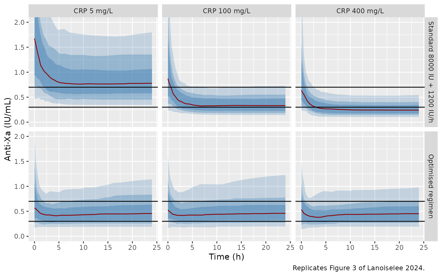
The medians at the start and the end of the 24 h course are compared below with values digitised by the maintainers from Figure 3 (read to about 0.05 IU/mL).
fig3_digit <- tibble(
  panel = rep(c("Standard 8000 IU + 1200 IU/h", "Optimised regimen"), each = 3),
  CRP = rep(c(5, 100, 400), 2),
  paper_t0 = c(1.60, 0.90, 0.70, 0.52, 0.45, 0.48),
  paper_t24 = c(0.72, 0.35, 0.25, 0.45, 0.42, 0.42)
)
fig3_sim <- pct |>
  filter(time %in% c(0, 24)) |>
  mutate(CRP = as.numeric(sub("CRP ([0-9]+) mg/L", "\\1", CRP)),
         panel = as.character(panel)) |>
  select(panel, CRP, time, q50) |>
  pivot_wider(names_from = time, values_from = q50, names_prefix = "sim_t")
fig3_cmp <- inner_join(fig3_digit, fig3_sim, by = c("panel", "CRP")) |>
  mutate(pct_t0 = 100 * (sim_t0 / paper_t0 - 1),
         pct_t24 = 100 * (sim_t24 / paper_t24 - 1))
fig3_cmp |>
  dplyr::rename(
    "Regimen" = panel, "CRP (mg/L)" = CRP,
    "Paper median t = 0" = paper_t0, "Simulated median t = 0" = sim_t0,
    "Paper median t = 24 h" = paper_t24, "Simulated median t = 24 h" = sim_t24,
    "% diff t = 0" = pct_t0, "% diff t = 24 h" = pct_t24
  ) |>
knitr::kable(digits = 2)| Regimen | CRP (mg/L) | Paper median t = 0 | Paper median t = 24 h | Simulated median t = 0 | Simulated median t = 24 h | % diff t = 0 | % diff t = 24 h |
|---|---|---|---|---|---|---|---|
| Standard 8000 IU + 1200 IU/h | 5 | 1.60 | 0.72 | 1.67 | 0.78 | 4.64 | 8.07 |
| Standard 8000 IU + 1200 IU/h | 100 | 0.90 | 0.35 | 0.87 | 0.33 | -3.16 | -5.13 |
| Standard 8000 IU + 1200 IU/h | 400 | 0.70 | 0.25 | 0.64 | 0.24 | -8.77 | -3.41 |
| Optimised regimen | 5 | 0.52 | 0.45 | 0.57 | 0.46 | 9.27 | 1.30 |
| Optimised regimen | 100 | 0.45 | 0.42 | 0.53 | 0.46 | 16.95 | 9.54 |
| Optimised regimen | 400 | 0.48 | 0.42 | 0.53 | 0.45 | 11.12 | 7.71 |
Figure 2: covariate-adjusted loading and maintenance doses
Replicates Figure 2 of Lanoiselee 2024: the dose needed to reach 0.5
IU/mL as a function of body weight (loading dose) or serum creatinine
(maintenance dose). Because the doses are V x T and
CL x T and both parameters are log-normal, the 50%, 70% and
90% interpatient intervals follow directly from the IIV standard
deviations. Points: medians digitised by the maintainers from the
figure.
z <- qnorm(c(0.05, 0.15, 0.25, 0.75, 0.85, 0.95))
sd_v <- sqrt(0.5625)
sd_cl <- sqrt(0.2704)
band <- function(med, sd) {
  q <- outer(med, exp(z * sd))
  tibble(med = med, q05 = q[, 1], q15 = q[, 2], q25 = q[, 3],
         q75 = q[, 4], q85 = q[, 5], q95 = q[, 6])
}

ld_curve <- tidyr::crossing(wt = seq(50, 150, by = 2), crp = c(5, 100, 400),
                            postcard = c(0, 1)) |>
  mutate(med = typ_v(wt, crp, postcard) * target)
ld_curve <- bind_cols(ld_curve |> select(-med), band(ld_curve$med, sd_v)) |>
  mutate(row = ifelse(postcard == 1, "LD, post-cardiotomy", "LD, medical"),
         x = wt)
md_curve <- tidyr::crossing(creat = seq(25, 500, by = 5), crp = c(5, 100, 400)) |>
  mutate(med = typ_cl(creat, crp) * target)
md_curve <- bind_cols(md_curve |> select(-med), band(md_curve$med, sd_cl)) |>
  mutate(row = "MD (IU/h)", x = creat)

fig2_digit <- tibble(
  row = c(rep("LD, medical", 3), rep("MD (IU/h)", 3)),
  crp = rep(c(5, 100, 400), 2),
  x = c(150, 150, 150, 500, 500, 500),
  paper = c(4460, 8000, 10500, 490, 1060, 1520)
)

curves <- bind_rows(ld_curve, md_curve) |>
  mutate(crp = factor(paste("CRP", crp, "mg/L"), levels = paste("CRP", c(5, 100, 400), "mg/L")))
ggplot(curves, aes(x)) +
  geom_ribbon(aes(ymin = q05, ymax = q95), fill = "steelblue", alpha = 0.25) +
  geom_ribbon(aes(ymin = q15, ymax = q85), fill = "steelblue", alpha = 0.35) +
  geom_ribbon(aes(ymin = q25, ymax = q75), fill = "steelblue", alpha = 0.45) +
  geom_line(aes(y = med), colour = "darkred") +
  geom_point(data = fig2_digit |>
               mutate(crp = factor(paste("CRP", crp, "mg/L"),
                                   levels = paste("CRP", c(5, 100, 400), "mg/L"))),
             aes(y = paper), shape = 4, size = 3) +
  scale_y_log10() +
  facet_grid(row ~ crp, scales = "free") +
  labs(x = "Body weight (kg) for LD; serum creatinine (umol/L) for MD",
       y = "Dose for a 0.5 IU/mL target (IU or IU/h)",
       caption = "Replicates Figure 2 of Lanoiselee 2024; crosses are digitised medians.")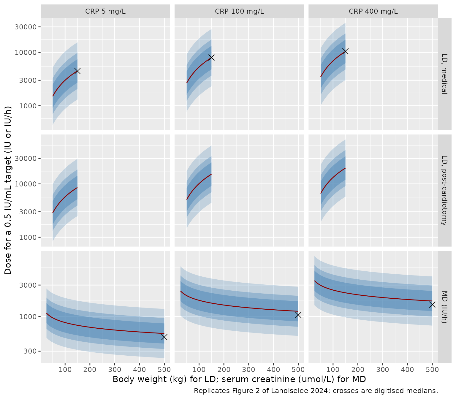
fig2_cmp <- fig2_digit |>
  mutate(model = ifelse(row == "LD, medical",
                        typ_v(x, crp, 0) * target,
                        typ_cl(x, crp) * target),
         pct_diff = 100 * (model / paper - 1))
fig2_cmp |>
  dplyr::rename("Curve" = row, "CRP (mg/L)" = crp, "BW (kg) or SCr (umol/L)" = x,
                "Paper (digitised)" = paper, "Model" = model, "% diff" = pct_diff) |>
knitr::kable(digits = 0)| Curve | CRP (mg/L) | BW (kg) or SCr (umol/L) | Paper (digitised) | Model | % diff |
|---|---|---|---|---|---|
| LD, medical | 5 | 150 | 4460 | 4493 | 1 |
| LD, medical | 100 | 150 | 8000 | 7963 | 0 |
| LD, medical | 400 | 150 | 10500 | 10377 | -1 |
| MD (IU/h) | 5 | 500 | 490 | 556 | 13 |
| MD (IU/h) | 100 | 500 | 1060 | 1204 | 14 |
| MD (IU/h) | 400 | 500 | 1520 | 1721 | 13 |
ld_rows <- fig2_cmp$row == "LD, medical"
# Loading doses: same formula on both sides, so only digitisation error.
stopifnot(all(abs(fig2_cmp$pct_diff[ld_rows]) < 8))
# Maintenance doses: the CRP ratios the figure implies match the CRP exponent.
md <- fig2_cmp[!ld_rows, ]
stopifnot(abs((md$paper[3] / md$paper[2]) / (md$model[3] / md$model[2]) - 1) < 0.08)
The loading-dose medians match the packaged volume to within
digitisation error, including the post-cardiotomy factor exp(0.647) =
1.91. The maintenance-dose medians share the packaged CRP and creatinine
dependence (the CRP ratios agree) but lie about 13% below
CL x 0.5 IU/mL across every panel. See Assumptions and
deviations.
Supplementary Figures S2-S4: indication, weight and creatinine
Typical-value anti-Xa under the optimised regimens of Supplementary Figures S2-S4 (all scenarios with CRP 100 mg/L). The rounded doses keep the typical anti-Xa inside 0.3-0.7 IU/mL over 24 h, as the paper reports.
supp_scen <- tribble(
  ~panel, ~scenario, ~WT, ~CREAT, ~ECMO_IND_POSTCARDIOTOMY, ~ld, ~md,
  "S2 indication", "Medical", 80, 115, 0, 4000, 1500,
  "S2 indication", "Post-cardiotomy", 80, 115, 1, 8000, 1500,
  "S3 weight", "50 kg", 50, 115, 0, 3000, 1500,
  "S3 weight", "80 kg", 80, 115, 0, 4000, 1500,
  "S3 weight", "120 kg", 120, 115, 0, 7000, 1500,
  "S4 creatinine", "SCr 25 umol/L", 80, 25, 0, 4000, 2000,
  "S4 creatinine", "SCr 115 umol/L", 80, 115, 0, 4000, 1500,
  "S4 creatinine", "SCr 500 umol/L", 80, 500, 0, 4000, 1000
) |>
  mutate(CRP = 100, id = row_number())
supp_ev <- bind_rows(
  supp_scen |> transmute(id, time = 0, amt = ld, rate = 0, evid = 1L, cmt = "central"),
  supp_scen |> transmute(id, time = 0, amt = md * 24, rate = md, evid = 1L, cmt = "central"),
  supp_scen |> select(id) |> tidyr::crossing(time = grid) |>
    mutate(amt = NA_real_, rate = NA_real_, evid = 0L, cmt = "central")
) |>
  left_join(supp_scen |> select(id, panel, scenario, WT, CREAT, CRP, ECMO_IND_POSTCARDIOTOMY),
            by = "id") |>
  arrange(id, time, desc(evid))
# A multi-subject typical-value solve has no omega; rxode2's note about that
# is expected and muffled.
supp_sim <- withCallingHandlers(
  rxode2::rxSolve(rxode2::zeroRe(mod), events = supp_ev,
                  returnType = "data.frame", keep = c("panel", "scenario")),
  warning = function(w) {
    if (grepl("without 'omega'", conditionMessage(w), fixed = TRUE)) {
      invokeRestart("muffleWarning")
    }
  }
)
#> ℹ parameter labels from comments will be replaced by 'label()'
#> ℹ omega/sigma items treated as zero: 'etalcl', 'etalvc'

ggplot(supp_sim, aes(time, Cc, colour = scenario)) +
  geom_line() +
  geom_hline(yintercept = c(0.3, 0.7)) +
  facet_wrap(~panel) +
  coord_cartesian(ylim = c(0, 1)) +
  labs(x = "Time (h)", y = "Typical anti-Xa (IU/mL)", colour = NULL,
       caption = "Typical-value replication of the bottom panels of Supplementary Figures S2-S4.")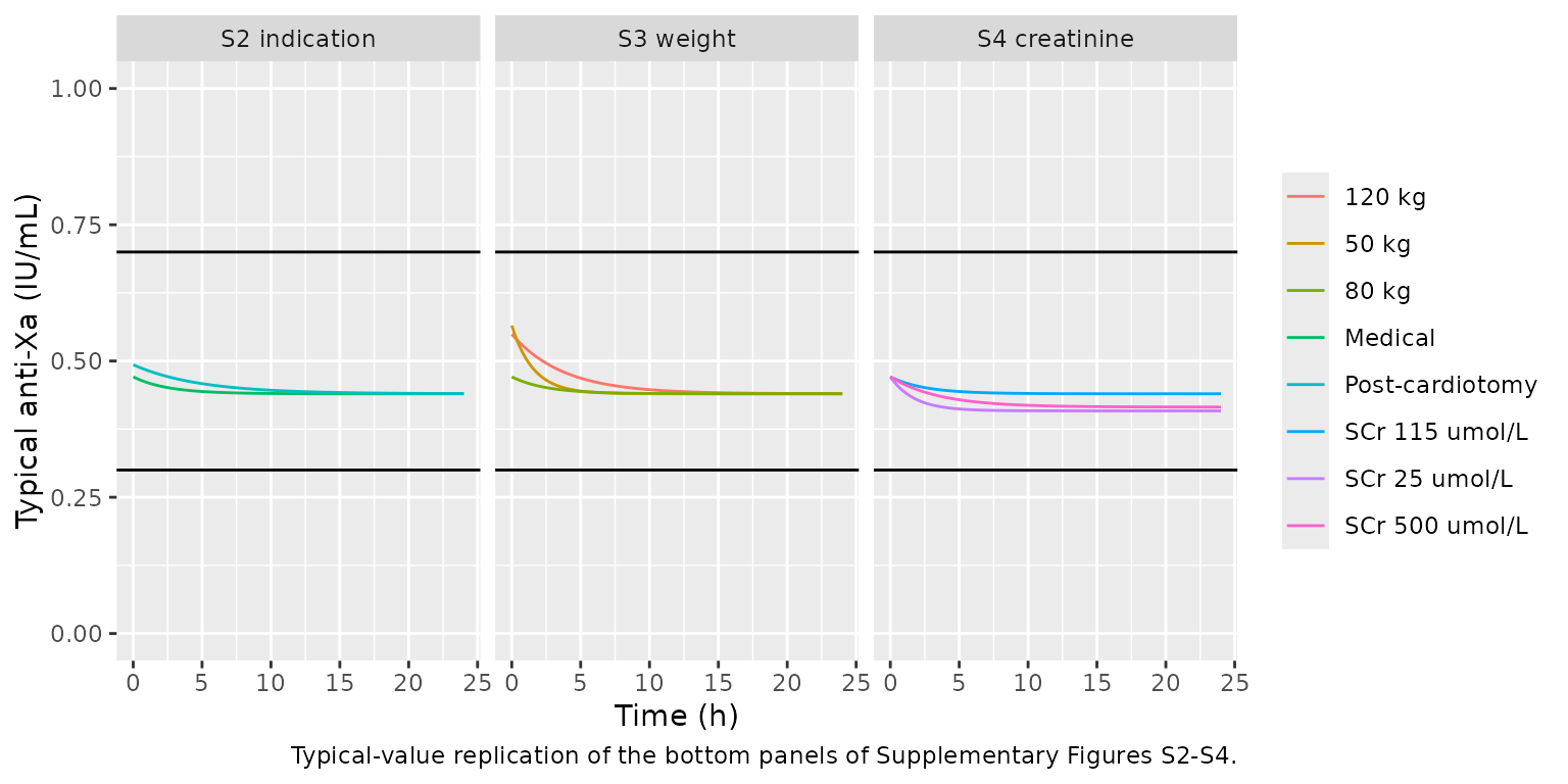
PKNCA validation
Lanoiselee 2024 reports no non-compartmental results, so the NCA check is one of internal consistency: PKNCA AUC0-24 on the simulated Figure 3 cohort is compared, subject by subject, with the closed-form AUC of a bolus plus a constant-rate infusion into one compartment.
sim_nca <- sim |>
  filter(!is.na(Cc)) |>
  select(id, time, Cc, scenario)
dose_df <- events |>
  filter(evid == 1) |>
  group_by(id, scenario) |>
  summarise(time = 0, amt = sum(amt), .groups = "drop")

conc_obj <- PKNCA::PKNCAconc(sim_nca, Cc ~ time | scenario + id)
dose_obj <- PKNCA::PKNCAdose(dose_df, amt ~ time | scenario + id, route = "intravascular")
intervals <- data.frame(start = 0, end = 24, cmax = TRUE, auclast = TRUE, cav = TRUE)
nca_res <- PKNCA::pk.nca(PKNCA::PKNCAdata(conc_obj, dose_obj, intervals = intervals))

nca_res$result |>
  as.data.frame() |>
  filter(PPTESTCD %in% c("cmax", "auclast", "cav")) |>
  group_by(scenario, PPTESTCD) |>
  summarise(median = median(PPORRES), .groups = "drop") |>
  pivot_wider(names_from = PPTESTCD, values_from = median) |>
  dplyr::rename("Scenario" = scenario, "Cmax (IU/mL)" = cmax,
                "AUC0-24 (IU*h/mL)" = auclast, "Cavg 0-24 (IU/mL)" = cav) |>
knitr::kable(digits = 2, caption = "Median simulated NCA parameters by scenario.")| Scenario | AUC0-24 (IU*h/mL) | Cavg 0-24 (IU/mL) | Cmax (IU/mL) |
|---|---|---|---|
| Optimised regimen, CRP 100 mg/L | 10.67 | 0.44 | 0.69 |
| Optimised regimen, CRP 400 mg/L | 10.78 | 0.45 | 0.67 |
| Optimised regimen, CRP 5 mg/L | 10.44 | 0.44 | 0.75 |
| Standard 8000 IU + 1200 IU/h, CRP 100 mg/L | 9.13 | 0.38 | 0.88 |
| Standard 8000 IU + 1200 IU/h, CRP 400 mg/L | 6.72 | 0.28 | 0.66 |
| Standard 8000 IU + 1200 IU/h, CRP 5 mg/L | 19.80 | 0.82 | 1.80 |
params <- sim |>
  filter(time == 0) |>
  distinct(id, cl, vc, ld, md) |>
  mutate(
    k = cl / vc,
    auc_cf = (ld / cl * (1 - exp(-24 * k)) +
                md / cl * (24 - (1 - exp(-24 * k)) / k)) / 1000
  )
auc_chk <- nca_res$result |>
  as.data.frame() |>
  filter(PPTESTCD == "auclast") |>
  select(id, auc = PPORRES) |>
  inner_join(params, by = "id") |>
  mutate(pct_diff = 100 * (auc / auc_cf - 1))
stopifnot(nrow(auc_chk) == nrow(fig3_scen) * n_per)
# Same drawn parameters on both sides: the gap is trapezoidal error on a
# 0.25 h grid, largest for fast-eliminating subjects right after the bolus.
stopifnot(
  abs(median(auc_chk$pct_diff)) < 1,
  quantile(abs(auc_chk$pct_diff), 0.9) < 3
)
Assumptions and deviations
-
ECMO-indication term on V. Table 2 prints the
volume as
theta4^(Indic x theta5) x ..., which would give a volume of 1 L for every medical patient. The Section 3.3 loading-dose equation writes the same term asexp(Indic x theta_Indic), and that form reproduces Figure 2 (the post-cardiotomy loading doses are 1.91-fold the medical ones) and Supplementary Figure S2 (4000 versus 8000 IU). The packaged model usesV = 8.65 * exp(0.647 * ECMO_IND_POSTCARDIOTOMY) * (WT/80) * (CRP/110)^0.191. - CRP centring on V. Table 2 centres CRP on 110 mg/L for V and on 100 mg/L for CL; the Section 3.3 loading-dose equation and the Section 3.4 text use 100 mg/L. The maintainers kept the Table 2 value of 110 mg/L for V (the development-cohort median was 113 mg/L). The difference is 1.8% in the typical volume; the digitised loading doses of Figure 2 fit 110 marginally better.
- theta5 has no reported RSE. It is encoded as an estimated parameter, because Table 2 marks only theta6 as fixed.
-
Maintenance doses in Figure 2 and Figure 3. The
paper’s maintenance-dose curves are about 13% below
CL x 0.5 IU/mLcomputed from Table 2, at every CRP and creatinine level, while the loading-dose curves matchV x 0.5 IU/mL. The paper does not explain the offset, and the packaged clearance is not changed to absorb it. The anti-Xa simulations in Figure 3 agree with the packaged clearance. - Time-varying covariates. CRP and serum creatinine were time-varying in the fit (Section 2.6). The simulations here hold them constant, as the paper’s own simulations do. Users simulating real patients can supply them as time-varying columns in the event table.
- Censoring. Anti-Xa values below 0.1 IU/mL and above 1.8 IU/mL were handled as censored observations in the fit; the simulated anti-Xa is not censored.
-
Covariates tested but not retained (age,
fibrinogen, continuous renal replacement therapy) are listed in the
model’s
covariatesDataExcluded.