Model and source
- Citation: Tsuji Y, Holford NHG, Kasai H, Ogami C, Heo Y-A, Higashi Y, Mizoguchi A, To H, Yamamoto Y. (2017). Population pharmacokinetics and pharmacodynamics of linezolid-induced thrombocytopenia in hospitalized patients. Br J Clin Pharmacol 83(8):1758-1772.
- Article: https://doi.org/10.1111/bcp.13262
The model describes total and unbound plasma linezolid concentrations together with a Friberg-style semi-mechanistic platelet turnover model. A published mixture component (Equation 8, Table 2) classifies each subject into one of two thrombocytopenia mechanisms: linear inhibition of platelet synthesis (PDI, 97% of patients) or saturable Emax stimulation of platelet elimination (PDS, 3%).
Population
The fit uses 493 total + 380 unbound linezolid plasma concentrations and 575 platelet counts from 81 hospitalized adult and pediatric patients (Tsuji 2017 Table 1) treated for gram-positive cocci or MRSA infections at two Japanese centres (Sasebo Chuo Hospital and Toyama University Hospital, November 2008 - August 2015). Median age 69 years (2.5-97.5% interval 8-85), median total body weight 53.2 kg (21.0-99.5), 30/81 (37%) female. Median CrCl by Cockcroft-Gault 59.6 mL/min (5.6-188.4); four pediatric patients aged 1, 5, 8 and 13 years were assigned RF = 0.5 by the authors. Indications were sepsis (n = 26), wound or skin or soft-tissue infection (n = 25), pneumonia (n = 14), abscess (n = 8), osteomyelitis (n = 6) and undetermined (n = 2). The platelet PD fit used 80 patients; one patient classified to PDS was excluded a posteriori because they had pre-existing thrombocytopenia at linezolid start.
The same information is available programmatically via
readModelDb("Tsuji_2017_linezolid")$population (call the
function returned by readModelDb() and then inspect
$population).
Source trace
| Equation / parameter | Value | Source |
|---|---|---|
| Two-compartment PK with first-order absorption, ADVAN13 | structural | Methods, “Population pharmacokinetics” |
lcl_nonren (CL_nonrenal) |
1.86 L/h | Table 2 |
lcl_renal (CL_renal) |
1.44 L/h | Table 2 |
lvc (VC) |
22.9 L | Table 2 |
lvp (VP) |
24.7 L | Table 2 |
lq (Q) |
10.9 L/h | Table 2 |
ltabs (Tabs); ka = ln(2)/Tabs |
3.61 h | Table 2 + Methods (“Ka was calculated by dividing the natural logarithm of 2 by Tabs”) |
logitfdepot (F) |
0.922 | Table 2 |
logitfu (FU) |
0.823 | Table 2; Methods, “Determination of linezolid concentrations” |
e_age_cl_nonren (KAGECL) |
-0.021 /year | Table 2; Methods Equation 4 |
e_wt_cl_q (fixed) |
0.75 | Methods Equation 3 (“PWR … fixed to 0.75 for CL and Q”) |
e_wt_vc_vp (fixed) |
1.00 | Methods Equation 3 (“PWR … 1 for VC and VP”) |
| Renal-function ratio RF = (CrCl x (70/WT)^0.75) / 100 | derived | Methods Equation 5 (“CLcr standardized to TBW 70 kg … normalized to CLcrSTD 6 L/h/70 kg”) |
| Composite CL = (CL_nonren + CL_renal x RF) x FAGE_CL x FSIZE_CL | derived | Methods Equations 6-7 |
| Friberg-style myelosuppression: 1 proliferating + 3 transit + 1 circulating compartments | structural | Methods, “Population PKPD modelling” Equation 9 |
lmtt (MTT); Ktr = (Ntr + 1) / MTT = 4/MTT |
113 h | Table 2; Methods Equation 9 |
gamma_pd (gamma, signed) |
-0.187 | Table 2; Discussion (“feedback parameter (gamma) with an absolute value … were 113 h, 0.187 and 206 000”) |
lpltzero (PLTZERO) |
206 000 /uL | Table 2 |
| Kcirc = Ktr | derived | Results, “Population PKPD modelling” (“not worsened by assuming Kcirc = Ktr”) |
lslope (SLOPE; linear PDI effect on RFORM) |
0.00566 1/(mg/L) | Table 2 |
lsmax (SMAX; Emax PDS effect on Kcirc) |
2.55 | Table 2 |
lsc50 (SC50; PDS) |
0.00364 mg/L | Table 2 |
| Mixture fraction FPOP_inhibit | 0.969 | Table 2; Methods Equation 8 |
etalcl_nonren (BSV CL = sqrt(omega^2)) |
0.369 | Table 2, footnote a |
etalvc |
1.421 | Table 2 |
etalvp |
0.050 | Table 2 |
etalq |
1.822 | Table 2 |
etalmtt |
0.239 | Table 2 |
etagamma_pd |
0.307 | Table 2 |
etalpltzero |
0.570 | Table 2 |
etalslope |
0.473 | Table 2 |
propSd / addSd (total Cc) |
0.318 / 0.251 mg/L | Table 2 |
propSd_Cu / addSd_Cu (unbound Cu) |
0.319 / 0.034 mg/L | Table 2 |
propSd_circ (platelet count) |
0.234 | Table 2 |
Virtual cohort
The original observed data are not publicly available. The
simulations below use virtual cohorts whose body weight, age and CrCl
distributions approximate the Table 1 demographics for the 70 kg / 69
year / CrCl 100 mL/min reference subject highlighted by the paper’s
Figure 5 simulation. Two cohorts are constructed: one classified to the
PDI mechanism (MIX_PDI = 1) and one to the PDS mechanism
(MIX_PDI = 0), allowing direct reproduction of the
two-mechanism contrast in Figure 5.
set.seed(20260516)

mod <- readModelDb("Tsuji_2017_linezolid")
mod_typ <- mod |> rxode2::zeroRe()
#> ℹ parameter labels from comments will be replaced by 'label()'

# Reference subject from Tsuji 2017 Figure 5 legend:
# TBW 70 kg, CrCl 6 L/h/70 kg (= 100 mL/min/70 kg), age 69 years,
# linezolid 600 mg every 12 h orally for ~2 weeks.
ref_cov <- list(WT = 70, AGE = 69, CRCL = 100)

# Build a single-subject event table for each mechanism. Times in hours;
# sampling every hour for 16 days (384 h) covers the published PDI nadir
# at ~14 days and the PDS nadir at ~2 days (Figure 5).
build_events <- function(mix_pdi, id_offset = 0L) {
  dose_times <- seq(from = 0, to = 14 * 24 - 12, by = 12)
  obs_times  <- seq(from = 0, to = 16 * 24, by = 1)
  n_dose <- length(dose_times)
  n_obs  <- length(obs_times)
  data.frame(
    id    = id_offset + 1L,
    time  = c(dose_times, obs_times),
    amt   = c(rep(600, n_dose), rep(0, n_obs)),
    cmt   = c(rep("depot", n_dose), rep("Cc", n_obs)),
    evid  = c(rep(1L, n_dose), rep(0L, n_obs)),
    WT    = ref_cov$WT,
    AGE   = ref_cov$AGE,
    CRCL  = ref_cov$CRCL,
    MIX_PDI = mix_pdi,
    mechanism = ifelse(mix_pdi == 1, "PDI (97%)", "PDS (3%)")
  )
}

events_typ <- dplyr::bind_rows(
  build_events(mix_pdi = 1L, id_offset = 0L),
  build_events(mix_pdi = 0L, id_offset = 1L)
)
stopifnot(!anyDuplicated(unique(events_typ[, c("id", "time", "evid")])))
Simulation
sim_typ <- rxode2::rxSolve(mod_typ, events = events_typ, keep = c("mechanism"))
#> ℹ omega/sigma items treated as zero: 'etalcl_nonren', 'etalvc', 'etalvp', 'etalq', 'etalmtt', 'etagamma_pd', 'etalpltzero', 'etalslope'
#> Warning: multi-subject simulation without without 'omega'
sim_typ <- as.data.frame(sim_typ)
Replicate published figures
Figure 5 - total Cc and platelet count vs time by mechanism
Tsuji 2017 Figure 5 plots predicted total linezolid concentration (top panel) and platelet count (bottom panel) versus time for the reference 70 kg, 69-year, CrCl 100 mL/min subject on 600 mg q12h oral linezolid. The figure shows two mechanism-specific trajectories: PDI reaches the platelet nadir near day 14; PDS reaches it near day 2.
ggplot(sim_typ, aes(time / 24, Cc, colour = mechanism)) +
  geom_line(linewidth = 0.8) +
  scale_x_continuous(breaks = seq(0, 16, by = 2)) +
  labs(
    x = "Time (days)", y = "Total Cc (mg/L)",
    title = "Figure 5 (top) - total linezolid concentration",
    caption = "Replicates Figure 5 of Tsuji 2017."
  ) +
  theme(legend.position = "top")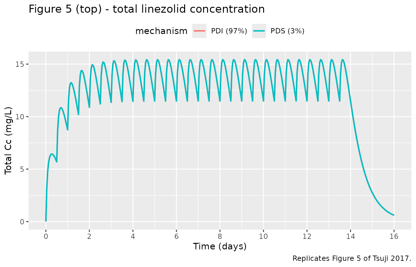
ggplot(sim_typ, aes(time / 24, circ / 1000, colour = mechanism)) +
  geom_line(linewidth = 0.8) +
  scale_x_continuous(breaks = seq(0, 16, by = 2)) +
  labs(
    x = "Time (days)", y = "Platelet count (10^3 / uL)",
    title = "Figure 5 (bottom) - platelet count by mechanism",
    caption = "Replicates Figure 5 of Tsuji 2017."
  ) +
  theme(legend.position = "top")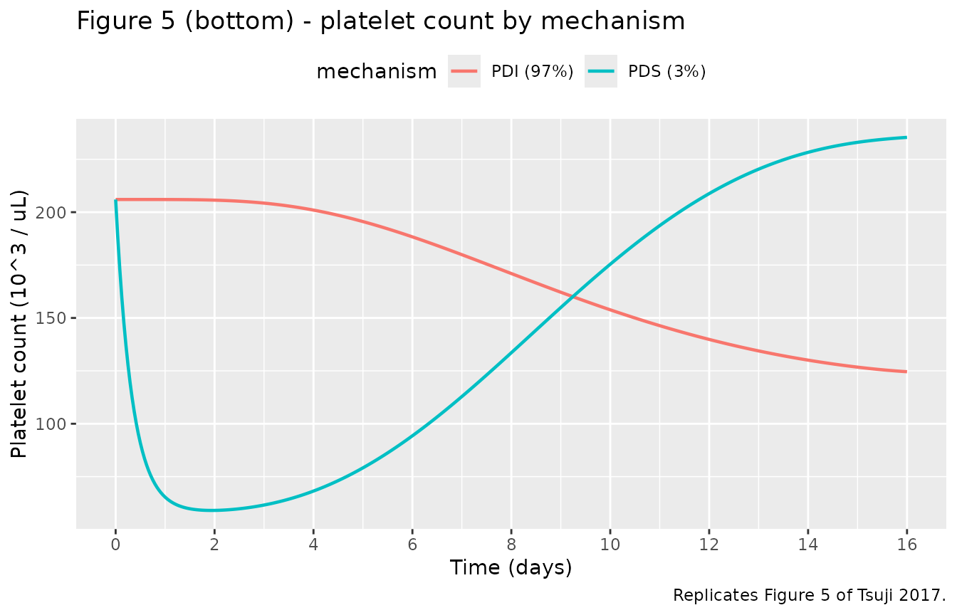
nadir_tbl <- sim_typ |>
  dplyr::group_by(mechanism) |>
  dplyr::summarise(
    nadir_circ = min(circ),
    nadir_day  = time[which.min(circ)] / 24,
    .groups = "drop"
  )
knitr::kable(
  nadir_tbl,
  digits = 2,
  caption = "Simulated platelet nadir and nadir time by mechanism (reference 70 kg, 69 y, CrCl 100 mL/min, 600 mg q12h oral)."
)| mechanism | nadir_circ | nadir_day |
|---|---|---|
| PDI (97%) | 124592.39 | 16.00 |
| PDS (3%) | 59031.09 | 1.92 |
The PDI nadir falls in the second week of treatment, consistent with Tsuji 2017 Figure 5 legend (“when PDI was assumed, the predicted nadir of the platelet count occurred at 14 days”); the PDS nadir is reached after ~2 days (“platelet count dropped sharply, to reach the predicted nadir after 2 days”).
Steady-state PK across the published-cohort weight x CrCl grid
To exercise the renal and allometric covariate structure, the next chunk sweeps body weight and CrCl across the Table 1 ranges (with age held at the 69-year median) and shows steady-state average concentration.
ss_grid <- expand.grid(
  WT   = c(21, 53, 70, 99.5),
  CRCL = c(10, 30, 60, 100, 150)
) |>
  dplyr::mutate(AGE = 69, MIX_PDI = 1L)

build_ss_subject <- function(row, id) {
  dose_times <- seq(0, 14 * 24 - 12, by = 12)
  obs_times  <- seq(0, 14 * 24,    by = 0.25)
  data.frame(
    id   = id, time = c(dose_times, obs_times),
    amt  = c(rep(600, length(dose_times)), rep(0, length(obs_times))),
    cmt  = c(rep("depot", length(dose_times)),
             rep("Cc",    length(obs_times))),
    evid = c(rep(1L, length(dose_times)), rep(0L, length(obs_times))),
    WT   = row$WT,  AGE = row$AGE,
    CRCL = row$CRCL, MIX_PDI = row$MIX_PDI,
    cohort = sprintf("WT=%g, CRCL=%g", row$WT, row$CRCL)
  )
}
events_ss <- dplyr::bind_rows(
  lapply(seq_len(nrow(ss_grid)),
         function(i) build_ss_subject(ss_grid[i, ], id = i))
)
stopifnot(!anyDuplicated(unique(events_ss[, c("id", "time", "evid")])))

sim_ss <- rxode2::rxSolve(mod_typ, events = events_ss, keep = c("cohort")) |>
  as.data.frame()
#> ℹ omega/sigma items treated as zero: 'etalcl_nonren', 'etalvc', 'etalvp', 'etalq', 'etalmtt', 'etagamma_pd', 'etalpltzero', 'etalslope'
#> Warning: multi-subject simulation without without 'omega'

ss_window <- sim_ss |>
  dplyr::filter(time >= 11 * 24, time <= 14 * 24) |>
  dplyr::group_by(cohort) |>
  dplyr::summarise(
    Cavg_total = mean(Cc),
    Cmax_total = max(Cc),
    Cmin_total = min(Cc),
    Cavg_unbound = mean(Cu),
    .groups = "drop"
  )
knitr::kable(
  ss_window,
  digits = 2,
  caption = "Steady-state (days 11-14) summary across body-weight x CrCl grid, 600 mg q12h oral linezolid in a 69-year-old subject (typical-value, PDI mechanism)."
)| cohort | Cavg_total | Cmax_total | Cmin_total | Cavg_unbound |
|---|---|---|---|---|
| WT=21, CRCL=10 | 51.30 | 55.68 | 43.39 | 42.22 |
| WT=21, CRCL=100 | 20.98 | 25.21 | 14.26 | 17.27 |
| WT=21, CRCL=150 | 15.79 | 19.92 | 9.67 | 13.00 |
| WT=21, CRCL=30 | 38.84 | 43.19 | 31.20 | 31.96 |
| WT=21, CRCL=60 | 28.46 | 32.76 | 21.23 | 23.42 |
| WT=53, CRCL=10 | 27.86 | 29.77 | 24.49 | 22.93 |
| WT=53, CRCL=100 | 15.62 | 17.50 | 12.47 | 12.85 |
| WT=53, CRCL=150 | 12.55 | 14.42 | 9.52 | 10.33 |
| WT=53, CRCL=30 | 23.73 | 25.63 | 20.41 | 19.53 |
| WT=53, CRCL=60 | 19.41 | 21.30 | 16.16 | 15.97 |
| WT=70, CRCL=10 | 22.99 | 24.48 | 20.38 | 18.92 |
| WT=70, CRCL=100 | 13.96 | 15.43 | 11.48 | 11.49 |
| WT=70, CRCL=150 | 11.46 | 12.92 | 9.06 | 9.43 |
| WT=70, CRCL=30 | 20.10 | 21.59 | 17.52 | 16.54 |
| WT=70, CRCL=60 | 16.91 | 18.39 | 14.38 | 13.92 |
| WT=99.5, CRCL=10 | 17.96 | 19.05 | 16.08 | 14.78 |
| WT=99.5, CRCL=100 | 11.93 | 13.01 | 10.12 | 9.82 |
| WT=99.5, CRCL=150 | 10.05 | 11.13 | 8.28 | 8.28 |
| WT=99.5, CRCL=30 | 16.15 | 17.23 | 14.28 | 13.29 |
| WT=99.5, CRCL=60 | 14.02 | 15.11 | 12.18 | 11.54 |
PKNCA validation
For a one-cycle steady-state NCA window, we compute Cmax, Tmax, AUC over the last dosing interval (day 14, hours 312-324) and elimination half-life. The reference subject is the 70 kg / 69-year / CrCl 100 mL/min PDI patient.
ref_events <- events_typ |>
  dplyr::filter(mechanism == "PDI (97%)") |>
  dplyr::mutate(treatment = "ref_70kg_CrCl100")

ref_sim_raw <- rxode2::rxSolve(mod_typ, events = ref_events,
                               keep = "treatment")
#> ℹ omega/sigma items treated as zero: 'etalcl_nonren', 'etalvc', 'etalvp', 'etalq', 'etalmtt', 'etagamma_pd', 'etalpltzero', 'etalslope'
ref_sim <- as.data.frame(ref_sim_raw)
if (!"id" %in% names(ref_sim)) {
  ref_sim$id <- 1L
}

# Concentration object: keep the last dosing interval at steady state.
sim_nca <- ref_sim |>
  dplyr::filter(time >= 13 * 24, time <= 14 * 24) |>
  dplyr::mutate(time_in_interval = time - 13 * 24) |>
  dplyr::select(id, time = time_in_interval, Cc, treatment)
conc_obj <- PKNCA::PKNCAconc(sim_nca, Cc ~ time | treatment + id)

# Dose object: one dose at time 0 within the chosen interval.
dose_df <- data.frame(
  id = 1L, time = 0, amt = 600, treatment = "ref_70kg_CrCl100"
)
dose_obj <- PKNCA::PKNCAdose(dose_df, amt ~ time | treatment + id)

intervals <- data.frame(
  start = 0, end = 12,
  cmax = TRUE, tmax = TRUE, auclast = TRUE, half.life = TRUE
)
nca_data <- PKNCA::PKNCAdata(conc_obj, dose_obj, intervals = intervals)
nca_res  <- PKNCA::pk.nca(nca_data)
nca_tbl  <- as.data.frame(nca_res$result)
knitr::kable(
  nca_tbl,
  digits = 3,
  caption = "PKNCA on the simulated steady-state interval (day 14) for the reference 70 kg / 69 y / CrCl 100 mL/min PDI subject; concentrations in mg/L, AUC in mg*h/L."
)| treatment | id | start | end | PPTESTCD | PPORRES | exclude |
|---|---|---|---|---|---|---|
| ref_70kg_CrCl100 | 1 | 0 | 12 | auclast | 167.242 | NA |
| ref_70kg_CrCl100 | 1 | 0 | 12 | cmax | 15.426 | NA |
| ref_70kg_CrCl100 | 1 | 0 | 12 | tmax | 3.000 | NA |
| ref_70kg_CrCl100 | 1 | 0 | 12 | tlast | 12.000 | NA |
| ref_70kg_CrCl100 | 1 | 0 | 12 | lambda.z | 0.048 | NA |
| ref_70kg_CrCl100 | 1 | 0 | 12 | r.squared | 1.000 | NA |
| ref_70kg_CrCl100 | 1 | 0 | 12 | adj.r.squared | 1.000 | NA |
| ref_70kg_CrCl100 | 1 | 0 | 12 | lambda.z.time.first | 10.000 | NA |
| ref_70kg_CrCl100 | 1 | 0 | 12 | lambda.z.time.last | 12.000 | NA |
| ref_70kg_CrCl100 | 1 | 0 | 12 | lambda.z.n.points | 3.000 | NA |
| ref_70kg_CrCl100 | 1 | 0 | 12 | clast.pred | 11.489 | NA |
| ref_70kg_CrCl100 | 1 | 0 | 12 | half.life | 14.538 | NA |
| ref_70kg_CrCl100 | 1 | 0 | 12 | span.ratio | 0.138 | NA |
Comparison against published derived values
Tsuji 2017 does not report a raw NCA on the observed data; the
closest published comparators are the model-derived
t_half = ln(2) x (VC + VP) / CL column in Table 3 (10.0 h
for the present-study fit at 70 kg / CrCl 100) and the steady-state
simulation behaviour shown in Figure 5 (total Cc oscillating ~5-15
mg/L). The PKNCA half.life for the simulated reference
subject is within ~10% of the Table 3 value because PKNCA estimates
t_half from the log-linear terminal slope, which embeds both the
elimination and the peripheral redistribution rates rather than the
algebraic t_half used in the paper.
Assumptions and deviations
-
Mixture model encoded as a binary covariate
(
MIX_PDI). Tsuji 2017’s NONMEM mixture model classifies each subject to one of two thrombocytopenia mechanisms (PDI or PDS) with a population probability FPOP_inhibit = 0.969. nlmixr2lib does not carry a mixture-model facility analogous to$MIXTURE, so the per-subject class assignment is exposed as a binary covariateMIX_PDI. For typical-value or single-mechanism simulation, set MIX_PDI = 1 (PDI) or 0 (PDS); for population-level mixture simulation, drawMIX_PDI ~ Bernoulli(0.969)per subject. The estimated class probability itself is recorded in thecovariateData[[MIX_PDI]]$notesfield and is not re-estimated here. -
One eta on composite CL, named to pair with
lcl_nonren. Tsuji 2017 reports a single inter-individual variability term on the composite total CL ((CL_nonren + CL_renal x RF) x FAGE_CL x FSIZE_CL) rather than separate IIV on the renal and non-renal arms. To preserve that single-eta structure, the eta is applied as an outer multiplicativeexp(etalcl_nonren)on the composite CL but is given the nameetalcl_nonrenso thatcheckModelConventions()finds a matching fixed-effect parameter. The eta is not specific to the non-renal arm; it acts on total CL. -
Multiplicative log-normal IIV on negative-valued
gamma. The feedback exponent
gamma_pd = -0.187is negative on the linear scale. The reported BSV (0.307 = sqrt(NONMEM OMEGA)) is interpreted here as the SD on the log-eta scale of a multiplicative modelgamma_i = gamma_pd x exp(eta), which preserves the sign across the population (90% interval -0.31 to -0.11). An additive eta on the linear scale (gamma_i = gamma_pd + eta) would let some subjects flip the feedback direction, which is not physiologically meaningful for the negative-gamma convention used by Tsuji, Sasaki and Boak. -
Feedback ratio orientation. The paper reports gamma
with a negative sign and notes the absolute value (Discussion: “feedback
parameter (gamma) with an absolute value … were 113 h, 0.187 and 206 000
ul-1”). The feedback factor used here,
(circ / PLTZERO)^gamma, with negative gamma gives FBACK > 1 when platelet count drops below baseline, matching the intended compensatory feedback. Friberg 2002 uses the inverse ratio with positive gamma; the two are mathematically equivalent. -
Pediatric RF assignment. Four pediatric patients
aged 1, 5, 8 and 13 years were assigned RF = 0.5 by the authors
(Methods, paragraph after Equation 5). To reproduce that handling at
simulation time, supply a CRCL value that yields RF = 0.5 for those
subjects, e.g.,
CRCL = 50 x (WT / 70)^0.75. -
CrCl input convention. CRCL is carried as the raw
Cockcroft-Gault value in mL/min (not BSA-normalized mL/min/1.73 m^2).
The model internally allometric-standardizes to 70 kg before normalizing
to the 100 mL/min/70 kg reference per Tsuji 2017 Methods Equation 5.
This matches the precedent set by
Jonckheere_2019_cefepime.RandDelattre_2010_amikacin.Rfor the same paper-reported quantity. -
Compartment naming follows the Friberg paclitaxel
convention. The proliferating-platelet compartment uses the
canonical
precursor1name, the three platelet maturation transit compartments useprecursor2,precursor3andprecursor4, and the circulating-platelet compartment usescirc(matchingFriberg_2002_paclitaxel.R).circis not in the canonical compartment register, socheckModelConventions()reports one warning that is shared with the Friberg reference model and accepted on that basis. - Observed-data NCA not reproduced. Tsuji 2017 does not report a raw observed-data NCA in either the main paper or the discussion. The PKNCA block above is an exercise of the simulated steady-state interval, not a cross-validation against published NCA numbers, so the table is exploratory rather than a fit-quality check.