Leritrelvir (Wang 2024)
Source:vignettes/articles/Wang_2024_leritrelvir.Rmd
Wang_2024_leritrelvir.RmdModel and source
ui <- rxode2::rxode(readModelDb("Wang_2024_leritrelvir"))
#> ℹ parameter labels from comments will be replaced by 'label()'
#> Warning: some etas defaulted to non-mu referenced, possible parsing error: etaiov_cl_1, etaiov_cl_2, etaiov_vc_1, etaiov_vc_2
#> as a work-around try putting the mu-referenced expression on a simple line- Citation: Wang K, Li H, Li Y, Xu F, Sun Z, Yang Y, Huang J, Chen X. Model informed dose regimen optimizing in development of leritrelvir for the treatment of mild or moderate COVID-19. Front Pharmacol. 2024;15:1449583. doi:10.3389/fphar.2024.1449583
- Description: Two-compartment population PK model for oral leritrelvir (RAY1216), a SARS-CoV-2 3CL protease inhibitor, given alone or with 100 mg ritonavir in healthy Chinese adults. Sequential zero-order input into the depot after an absorption lag, then first-order absorption; every structural parameter has a separate typical value with and without ritonavir. Female sex lowers CL/F, food raises F1, ka and the zero-order duration, and in repeated-dose regimens CL/F steps down 12 h after the first dose (auto-inhibition) and back up 96 h after it (auto-induction), with occasion-gated random effects on CL/F and Vc/F.
- Article: https://doi.org/10.3389/fphar.2024.1449583 (open access; the NONMEM control stream and supplementary Tables S1-S3 are in Supplementary Material 1)
Leritrelvir (RAY1216) is an oral SARS-CoV-2 3CL (main) protease inhibitor metabolised mainly by CYP3A. Wang 2024 pooled the first-in-human phase I study (NCT05829551), in which leritrelvir was given alone or boosted with 100 mg ritonavir, and used the resulting population PK model to choose between 400 mg three times daily (TID) alone and twice-daily (BID) dosing with ritonavir. The 400 mg TID monotherapy regimen was taken into phase II and III.
Population
72 healthy Chinese adults (Wang 2024 Table 1): median age 35 years (19-48), median weight 60.6 kg (48.2-90.8), median BMI 22.9 kg/m^2, 50% female, median creatinine clearance 115 mL/min. 1571 plasma concentrations were analysed (150 of 1721, 8.72%, were below the LLOQ and excluded). The study (Figure 1) had single-ascending-dose arms of 400, 800 and 1600 mg alone; a 200 mg alone then 200 mg + ritonavir crossover; an 800 mg (alone) and a 500 mg + ritonavir fasted/fed crossover; 300, 500 and 700 mg + ritonavir BID; and 400 mg TID alone. The multiple-dose arms dosed for 4 days plus a single morning dose on day 5. Each crossover subject was coded as two NONMEM IDs (102 IDs in total).
str(ui$population)
#> List of 14
#>  $ species       : chr "human"
#>  $ n_subjects    : num 72
#>  $ n_studies     : num 1
#>  $ age_range     : chr "19-48 years"
#>  $ age_median    : chr "35 years"
#>  $ weight_range  : chr "48.2-90.8 kg"
#>  $ weight_median : chr "60.6 kg"
#>  $ sex_female_pct: num 50
#>  $ race_ethnicity: chr "Chinese (single-country phase I study in China; race not tabulated)"
#>  $ disease_state : chr "Healthy adult volunteers"
#>  $ dose_range    : chr "Leritrelvir alone: 400, 800 and 1600 mg single dose; 200 mg single dose (DDI period 1); 800 mg single dose fast"| __truncated__
#>  $ regions       : chr "China"
#>  $ n_observations: num 1571
#>  $ notes         : chr "Phase I SAD / MAD / food-effect / DDI study NCT05829551 (Wang 2024 Figure 1, Table 1). 1571 leritrelvir plasma "| __truncated__
Source trace
| Model element | Value | Source |
|---|---|---|
| Structure: 2-compartment, first-order elimination | ADVAN4 TRANS4 | Results 3.2.1; supplement control stream |
| Sequential zero-order (D1) then first-order (Ka) absorption, with lag |
dur(depot), alag(depot)
|
Results 3.2.1; Discussion; control stream D1,
ALAG1
|
| Separate typical values alone vs with ritonavir | IF (RTV.EQ.0) |
Results 3.2.1; control stream |
lcl, lcl_boosted
|
44.4, 12.2 L/h | Table 2 CL Mono / Comb |
lvc, lvc_boosted
|
18.9, 9.78 L | Table 2 Vc Mono / Comb |
lka, lka_boosted
|
0.293, 0.169 1/h | Table 2 Ka Mono / Comb |
lq, lq_boosted
|
5.57, 0.611 L/h | Table 2 Q Mono / Comb |
lvp, lvp_boosted
|
58.2, 9.30 L | Table 2 Vp Mono / Comb |
ld1, ld1_boosted
|
0.0722, 0.0684 h | Table 2 D1 Mono / Comb |
ltlag, ltlag_boosted
|
0.189, 0.166 h | Table 2 ALAG1 Mono / Comb |
lfdepot |
log(1), fixed | Table 2 F1 = 1 FIX |
e_fed_fdepot |
0.409 | Results 3.2.1 F1 equation; Table 2 F1.FED = 1.51 |
e_fed_ka |
0.291 | Results 3.2.1 Ka equation; control stream THETA(17) |
e_fed_d1 |
3.14 | Results 3.2.1 D1 equation; control stream THETA(16) |
e_sexf_cl |
-0.224 | Results 3.2.1 CL equation; Table 2 CL.sex = 0.800 |
e_occ1_cl |
-0.469 | Results 3.2.1 CL equation; Table 2 CL.OC1.INH = 0.626 |
e_occ2_cl |
0.412 | Results 3.2.1 CL equation; Table 2 CL.OC2.IND = 1.51 |
| Occasion indicators OC1 (t >= 12 h), OC2 (t >= 96 h), multiple-dose only |
oc1, oc2
|
Control stream IF (DOSESCH.GT.1.AND.TIME.GE.12)
|
etalcl, etalvc, etalka,
etalvp, etald1
|
30.6, 80.8, 26.1, 44.7, 155% | Table 2 IIV; variance = (IIV%/100)^2 |
etaiov_cl_1, etaiov_cl_2
|
19.3% | Table 2 OC1.CL (OC2.CL blank: SAME) |
etaiov_vc_1, etaiov_vc_2
|
54.4% | Table 2 OC1.Vc (OC2.Vc blank: SAME) |
propSd |
0.244 | Table 2 proportional residual 24.4% |
propSd_fedearly (fed, <= 2 h after dose) |
0.702 | Table 2; control stream
IF (TFDS.LE.2.AND.FED.EQ.1)
|
| Concentration scaling |
Cc = 1000 * central / vc (ng/mL) |
Control stream S2 = V2/1000
|
Typical-value behaviour
Single 400 mg doses of leritrelvir alone, and 200 mg with ritonavir,
for a typical male and female subject in the fasted and fed state. Every
dose record carries rate = -2, which is what makes rxode2
use the modelled zero-order duration dur(depot); without it
the dose would enter the depot as a bolus.
ui_typ <- rxode2::zeroRe(ui)
#> Warning: No sigma parameters in the model
#> Warning: some etas defaulted to non-mu referenced, possible parsing error: etaiov_cl_1, etaiov_cl_2, etaiov_vc_1, etaiov_vc_2
#> as a work-around try putting the mu-referenced expression on a simple line
grid_sd <- sort(unique(c(seq(0, 4, by = 0.05), seq(4.25, 72, by = 0.25))))

typ_ev <- tidyr::expand_grid(
  scen = 1:8,
  time = grid_sd
) |>
  mutate(evid = 0L, amt = 0, rate = 0, cmt = "central") |>
  bind_rows(tibble(scen = 1:8, time = 0, evid = 1L, rate = -2, cmt = "depot")) |>
  left_join(
    tibble(
      scen = 1:8,
      CONMED_RTV = rep(c(0L, 1L), each = 4),
      dose = rep(c(400, 200), each = 4),
      SEXF = rep(c(0L, 1L, 0L, 1L), 2),
      FED = rep(c(0L, 0L, 1L, 1L), 2)
    ),
    by = "scen"
  ) |>
  mutate(
    id = scen,
    amt = ifelse(evid == 1L, dose, 0),
    MULTI_DOSE = 0L
  ) |>
  arrange(id, time, desc(evid))

typ <- rxode2::rxSolve(ui_typ, typ_ev, returnType = "data.frame", addDosing = FALSE,
                       keep = c("CONMED_RTV", "SEXF", "FED", "dose")) |>
  mutate(
    Regimen = ifelse(CONMED_RTV == 1, "200 mg + ritonavir", "400 mg alone"),
    Subject = paste(ifelse(SEXF == 1, "female", "male"), ifelse(FED == 1, "fed", "fasted"))
  )
#> ℹ omega/sigma items treated as zero: 'etalcl', 'etalvc', 'etalka', 'etalvp', 'etald1', 'etaiov_cl_1', 'etaiov_cl_2', 'etaiov_vc_1', 'etaiov_vc_2'
#> Warning: multi-subject simulation without without 'omega'

ggplot(typ, aes(time, Cc, colour = Subject)) +
  geom_line() +
  facet_wrap(~Regimen) +
  scale_y_log10() +
  labs(x = "Time after dose (h)", y = "Leritrelvir (ng/mL)",
       title = "Typical single-dose profiles")
#> Warning in scale_y_log10(): log-10 transformation introduced infinite values.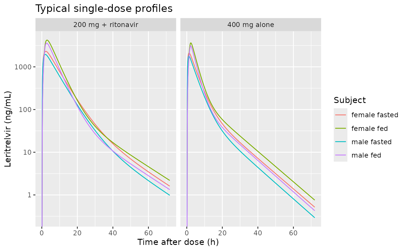
The zero-order duration is short in the fasted state (0.072 h) and
becomes 1.67 h with food (0.0722 * exp(3.14)). The check
below confirms rxode2 is spreading the fed dose over that window:
half-way through it, the depot must hold well under the full
bioavailable dose, whereas a bolus would leave about 80% of it
there.
d1_fed <- exp(log(0.0722) + 3.14)
t_mid <- 0.189 + d1_fed / 2
depot_mid <- typ |> filter(id == 3) |> slice(which.min(abs(time - t_mid))) |> pull(depot)
f_fed <- exp(0.409)
stopifnot(depot_mid < 0.6 * f_fed * 400)
c(d1_fed = d1_fed, depot_at_mid = depot_mid, bioavailable_dose = f_fed * 400)
#>            d1_fed      depot_at_mid bioavailable_dose
#>          1.668099        250.775374        602.124688
The AUC of a typical single dose must equal
F * dose / CL in closed form, which pins the clearance, the
bioavailability and the mg-to-ng/mL scaling.
typ_nca_conc <- typ |> filter(!is.na(Cc)) |> select(id, time, Cc, Regimen, Subject)
typ_nca_dose <- typ_ev |> filter(evid == 1L) |> select(id, time, amt)
typ_nca <- PKNCA::pk.nca(PKNCA::PKNCAdata(
  PKNCA::PKNCAconc(typ_nca_conc, Cc ~ time | Regimen + Subject + id),
  PKNCA::PKNCAdose(typ_nca_dose, amt ~ time | id),
  intervals = data.frame(start = 0, end = Inf, aucinf.obs = TRUE)
))
auc_closed <- typ_ev |>
  filter(evid == 1L) |>
  mutate(
    cl = ifelse(CONMED_RTV == 1, 12.2, 44.4) * exp(-0.224 * SEXF),
    auc_closed = 1000 * exp(0.409 * FED) * amt / cl
  ) |>
  select(id, auc_closed)
auc_cmp <- as.data.frame(typ_nca$result) |>
  filter(PPTESTCD == "aucinf.obs") |>
  left_join(auc_closed, by = "id") |>
  mutate(pct_diff = 100 * (PPORRES / auc_closed - 1))
auc_cmp |>
  select(Regimen, Subject, `AUCinf (ng*h/mL)` = PPORRES, `F*Dose/CL` = auc_closed, `% diff` = pct_diff) |>
knitr::kable(digits = 1)| Regimen | Subject | AUCinf (ng*h/mL) | F*Dose/CL | % diff |
|---|---|---|---|---|
| 200 mg + ritonavir | female fasted | 20508.1 | 20509.4 | 0 |
| 200 mg + ritonavir | female fed | 30871.1 | 30873.0 | 0 |
| 200 mg + ritonavir | male fasted | 16392.7 | 16393.4 | 0 |
| 200 mg + ritonavir | male fed | 24676.2 | 24677.2 | 0 |
| 400 mg alone | female fasted | 11270.8 | 11270.9 | 0 |
| 400 mg alone | female fed | 16966.3 | 16966.2 | 0 |
| 400 mg alone | male fasted | 9008.8 | 9009.0 | 0 |
| 400 mg alone | male fed | 13561.4 | 13561.4 | 0 |
Replicating Supplementary Table S1 and Figure 4
Wang 2024 simulated 1000 fasted subjects (500 male, 500 female) per
regimen: leritrelvir alone 300, 400, 500 and 600 mg TID (08:00, 14:00,
20:00) for five days, and 200 or 300 mg with ritonavir BID (08:00,
20:00), the BID arms taking a single morning dose on day 5 (the 9th
dose, Figure 4D). Here each arm has 200 subjects (100 male, 100 female).
The occasion indicators switch at 12 h and 96 h after the first dose
(MULTI_DOSE = 1).
The four occasion random effects (etaiov_*) are set to
zero for this replication. With them included, the simulated 10th-90th
percentile bands are much wider than the published ones at every time
after 12 h (the 90th percentile about 25% above the paper’s, up to 60%),
while with them excluded the bands agree to within a few percent at
every row of Table S1. The published simulation therefore appears to
carry only the between-subject variability. The occasion terms stay in
the model; they are set to zero only here.
n_per_arm <- 200
arms <- tibble(
  arm = 1:6,
  Regimen = c("300 mg TID", "400 mg TID", "500 mg TID", "600 mg TID",
              "300 mg BID + RTV", "200 mg BID + RTV"),
  dose = c(300, 400, 500, 600, 300, 200),
  CONMED_RTV = c(0L, 0L, 0L, 0L, 1L, 1L),
  tid = c(TRUE, TRUE, TRUE, TRUE, FALSE, FALSE)
)
dose_times_tid <- as.vector(outer(c(0, 6, 12), 24 * 0:4, "+"))
dose_times_bid <- seq(0, 96, by = 12)
obs_grid <- sort(unique(c(seq(0, 24, by = 0.25), seq(96, 120, by = 0.25))))

subjects <- tibble(arm = rep(arms$arm, each = n_per_arm)) |>
  mutate(id = row_number(), SEXF = rep(rep(c(0L, 1L), each = n_per_arm / 2), nrow(arms))) |>
  left_join(arms, by = "arm")

dose_rows <- bind_rows(
  tidyr::expand_grid(id = subjects$id[subjects$tid], time = dose_times_tid),
  tidyr::expand_grid(id = subjects$id[!subjects$tid], time = dose_times_bid)
) |>
  mutate(evid = 1L, rate = -2, cmt = "depot")
obs_rows <- tidyr::expand_grid(id = subjects$id, time = obs_grid) |>
  mutate(evid = 0L, rate = 0, cmt = "central")

ev_s1 <- bind_rows(dose_rows, obs_rows) |>
  left_join(subjects, by = "id") |>
  mutate(amt = ifelse(evid == 1L, dose, 0), FED = 0L, MULTI_DOSE = 1L) |>
  arrange(id, time, desc(evid)) |>
  select(id, time, evid, amt, rate, cmt, CONMED_RTV, SEXF, FED, MULTI_DOSE)

ui_noiov <- ui |>
  rxode2::ini(
    etaiov_cl_1 ~ 1e-10, etaiov_cl_2 ~ 1e-10,
    etaiov_vc_1 ~ 1e-10, etaiov_vc_2 ~ 1e-10
  )
#> ℹ change initial estimate of `etaiov_cl_1` to `1e-10`
#> ℹ change initial estimate of `etaiov_cl_2` to `1e-10`
#> ℹ change initial estimate of `etaiov_vc_1` to `1e-10`
#> ℹ change initial estimate of `etaiov_vc_2` to `1e-10`

rxode2::rxSetSeed(20240911)
sim_s1 <- rxode2::rxSolve(ui_noiov, ev_s1, returnType = "data.frame", addDosing = FALSE) |>
  left_join(select(subjects, id, Regimen), by = "id")
table_s1 <- tribble(
  ~Regimen,           ~dose_no, ~time, ~paper_med, ~paper_p10, ~paper_p90,
  "300 mg TID",        "1st",    6,    455,  269,  746,
  "300 mg TID",        "2nd",   12,    633,  373, 1019,
  "300 mg TID",        "3rd",   24,    311,  140,  650,
  "300 mg TID",        "13th", 102,    600,  332, 1017,
  "300 mg TID",        "14th", 108,    677,  375, 1148,
  "300 mg TID",        "15th", 120,    215,   96,  444,
  "400 mg TID",        "1st",    6,    624,  362, 1065,
  "400 mg TID",        "2nd",   12,    860,  491, 1447,
  "400 mg TID",        "3rd",   24,    436,  184,  976,
  "400 mg TID",        "13th", 102,    809,  448, 1508,
  "400 mg TID",        "14th", 108,    910,  501, 1711,
  "400 mg TID",        "15th", 120,    287,  119,  686,
  "500 mg TID",        "1st",    6,    762,  456, 1276,
  "500 mg TID",        "2nd",   12,   1035,  626, 1728,
  "500 mg TID",        "3rd",   24,    517,  245, 1124,
  "500 mg TID",        "13th", 102,    990,  562, 1750,
  "500 mg TID",        "14th", 108,   1115,  633, 1985,
  "500 mg TID",        "15th", 120,    343,  159,  761,
  "600 mg TID",        "1st",    6,    920,  569, 1528,
  "600 mg TID",        "2nd",   12,   1260,  771, 2106,
  "600 mg TID",        "3rd",   24,    633,  297, 1379,
  "600 mg TID",        "13th", 102,   1206,  713, 2138,
  "600 mg TID",        "14th", 108,   1360,  790, 2449,
  "600 mg TID",        "15th", 120,    426,  192,  942,
  "300 mg BID + RTV",  "1st",   12,    817,  446, 1395,
  "300 mg BID + RTV",  "2nd",   24,   1585,  807, 2862,
  "300 mg BID + RTV",  "9th",  108,   1047,  530, 2000,
  "200 mg BID + RTV",  "1st",   12,    543,  312,  911,
  "200 mg BID + RTV",  "2nd",   24,   1077,  561, 1889,
  "200 mg BID + RTV",  "9th",  108,    705,  366, 1320
)

s1_sim <- sim_s1 |>
  filter(time %in% table_s1$time) |>
  group_by(Regimen, time) |>
  summarise(
    sim_med = median(Cc),
    sim_p10 = quantile(Cc, 0.1),
    sim_p90 = quantile(Cc, 0.9),
    .groups = "drop"
  )
s1_cmp <- table_s1 |>
  left_join(s1_sim, by = c("Regimen", "time")) |>
  mutate(
    pct_med = 100 * (sim_med / paper_med - 1),
    pct_p10 = 100 * (sim_p10 / paper_p10 - 1),
    pct_p90 = 100 * (sim_p90 / paper_p90 - 1)
  )
stopifnot(nrow(s1_cmp) == 30, !anyNA(s1_cmp$sim_med))

s1_cmp |>
  transmute(
    Regimen, Dose = dose_no, `Time (h)` = time,
    `Paper median (P10-P90)` = sprintf("%.0f (%.0f-%.0f)", paper_med, paper_p10, paper_p90),
    `Simulated median (P10-P90)` = sprintf("%.0f (%.0f-%.0f)", sim_med, sim_p10, sim_p90),
    `% diff median` = round(pct_med, 1)
  ) |>
knitr::kable(caption = "Trough concentrations (ng/mL): Wang 2024 Supplementary Table S1 vs simulation.")| Regimen | Dose | Time (h) | Paper median (P10-P90) | Simulated median (P10-P90) | % diff median |
|---|---|---|---|---|---|
| 300 mg TID | 1st | 6 | 455 (269-746) | 472 (287-819) | 3.6 |
| 300 mg TID | 2nd | 12 | 633 (373-1019) | 594 (342-1114) | -6.1 |
| 300 mg TID | 3rd | 24 | 311 (140-650) | 315 (154-765) | 1.4 |
| 300 mg TID | 13th | 102 | 600 (332-1017) | 640 (373-1269) | 6.7 |
| 300 mg TID | 14th | 108 | 677 (375-1148) | 708 (401-1384) | 4.6 |
| 300 mg TID | 15th | 120 | 215 (96-444) | 216 (109-548) | 0.4 |
| 400 mg TID | 1st | 6 | 624 (362-1065) | 621 (342-1005) | -0.5 |
| 400 mg TID | 2nd | 12 | 860 (491-1447) | 776 (409-1336) | -9.8 |
| 400 mg TID | 3rd | 24 | 436 (184-976) | 450 (170-944) | 3.3 |
| 400 mg TID | 13th | 102 | 809 (448-1508) | 823 (432-1429) | 1.7 |
| 400 mg TID | 14th | 108 | 910 (501-1711) | 928 (477-1602) | 2.0 |
| 400 mg TID | 15th | 120 | 287 (119-686) | 299 (115-645) | 4.2 |
| 500 mg TID | 1st | 6 | 762 (456-1276) | 767 (448-1288) | 0.6 |
| 500 mg TID | 2nd | 12 | 1035 (626-1728) | 977 (530-1640) | -5.6 |
| 500 mg TID | 3rd | 24 | 517 (245-1124) | 537 (241-1142) | 3.9 |
| 500 mg TID | 13th | 102 | 990 (562-1750) | 1030 (566-1856) | 4.1 |
| 500 mg TID | 14th | 108 | 1115 (633-1985) | 1152 (632-2051) | 3.3 |
| 500 mg TID | 15th | 120 | 343 (159-761) | 365 (154-766) | 6.3 |
| 600 mg TID | 1st | 6 | 920 (569-1528) | 916 (568-1603) | -0.5 |
| 600 mg TID | 2nd | 12 | 1260 (771-2106) | 1125 (702-2064) | -10.7 |
| 600 mg TID | 3rd | 24 | 633 (297-1379) | 616 (305-1558) | -2.7 |
| 600 mg TID | 13th | 102 | 1206 (713-2138) | 1189 (727-2374) | -1.4 |
| 600 mg TID | 14th | 108 | 1360 (790-2449) | 1334 (816-2615) | -1.9 |
| 600 mg TID | 15th | 120 | 426 (192-942) | 420 (192-1008) | -1.5 |
| 300 mg BID + RTV | 1st | 12 | 817 (446-1395) | 812 (379-1383) | -0.6 |
| 300 mg BID + RTV | 2nd | 24 | 1585 (807-2862) | 1642 (726-2984) | 3.6 |
| 300 mg BID + RTV | 9th | 108 | 1047 (530-2000) | 1153 (498-2261) | 10.2 |
| 200 mg BID + RTV | 1st | 12 | 543 (312-911) | 503 (279-892) | -7.3 |
| 200 mg BID + RTV | 2nd | 24 | 1077 (561-1889) | 1049 (549-1896) | -2.6 |
| 200 mg BID + RTV | 9th | 108 | 705 (366-1320) | 704 (361-1403) | -0.2 |
c(
  median_pct_med = median(s1_cmp$pct_med),
  q90_abs_pct_med = unname(quantile(abs(s1_cmp$pct_med), 0.9)),
  median_abs_pct_p10 = median(abs(s1_cmp$pct_p10)),
  median_abs_pct_p90 = median(abs(s1_cmp$pct_p90))
)
#>     median_pct_med    q90_abs_pct_med median_abs_pct_p10 median_abs_pct_p90
#>          0.5241913          7.5599124          5.2211492          6.0358260
stopifnot(
  # Centre: a mis-transcribed clearance, volume or occasion step moves the
  # whole set of troughs by tens of percent.
  abs(median(s1_cmp$pct_med)) < 6,
  # Envelope over the 30 rows, robust to which subjects land in the tails.
  quantile(abs(s1_cmp$pct_med), 0.9) < 18,
  # Spread: the occasion effects left in would push the P90 ~25% high.
  median(abs(s1_cmp$pct_p90)) < 12
)
The medians agree with Table S1 to within a few percent across all 30
rows. The rows taken exactly at 12 h, the auto-inhibition boundary, tend
to come out below the paper (by up to about 11%). Concentrations there
are very sensitive to exactly when the clearance step takes effect,
because CL/Vc is about 2.3 1/h for leritrelvir alone (1.25
1/h with ritonavir), so plasma follows a clearance change within a
fraction of an hour. Small differences between how NONMEM and rxode2
time the switch around a record at 12 h are a plausible cause.
fig4 <- sim_s1 |>
  mutate(
    Day = ifelse(time <= 24, "Day 1", "Day 5"),
    tday = ifelse(time <= 24, time, time - 96)
  ) |>
  filter(!(Day == "Day 5" & grepl("BID", Regimen) & tday > 12)) |>
  group_by(Regimen, Day, tday) |>
  summarise(med = median(Cc), lo = quantile(Cc, 0.1), hi = quantile(Cc, 0.9), .groups = "drop") |>
  mutate(Panel = paste(ifelse(grepl("BID", Regimen), "BID with RTV", "TID without RTV"), "-", Day))

ggplot(fig4, aes(tday, med, colour = Regimen, fill = Regimen)) +
  geom_ribbon(aes(ymin = lo, ymax = hi), alpha = 0.15, colour = NA) +
  geom_line() +
  geom_hline(
    data = data.frame(ec90 = c(209.7, 165), lt = c("solid", "dashed")),
    aes(yintercept = ec90, linetype = I(lt)),
    colour = "darkgreen"
  ) +
  facet_wrap(~Panel, scales = "free_x") +
  scale_y_log10() +
  labs(x = "Time (h)", y = "Leritrelvir (ng/mL)",
       caption = "Replicates Figure 4 of Wang 2024: median and 10th-90th percentile; green lines are the EC90 targets 209.7 and 165 ng/mL.")
#> Warning in scale_y_log10(): log-10 transformation introduced infinite values.
#> log-10 transformation introduced infinite values.
#> log-10 transformation introduced infinite values.
#> log-10 transformation introduced infinite values.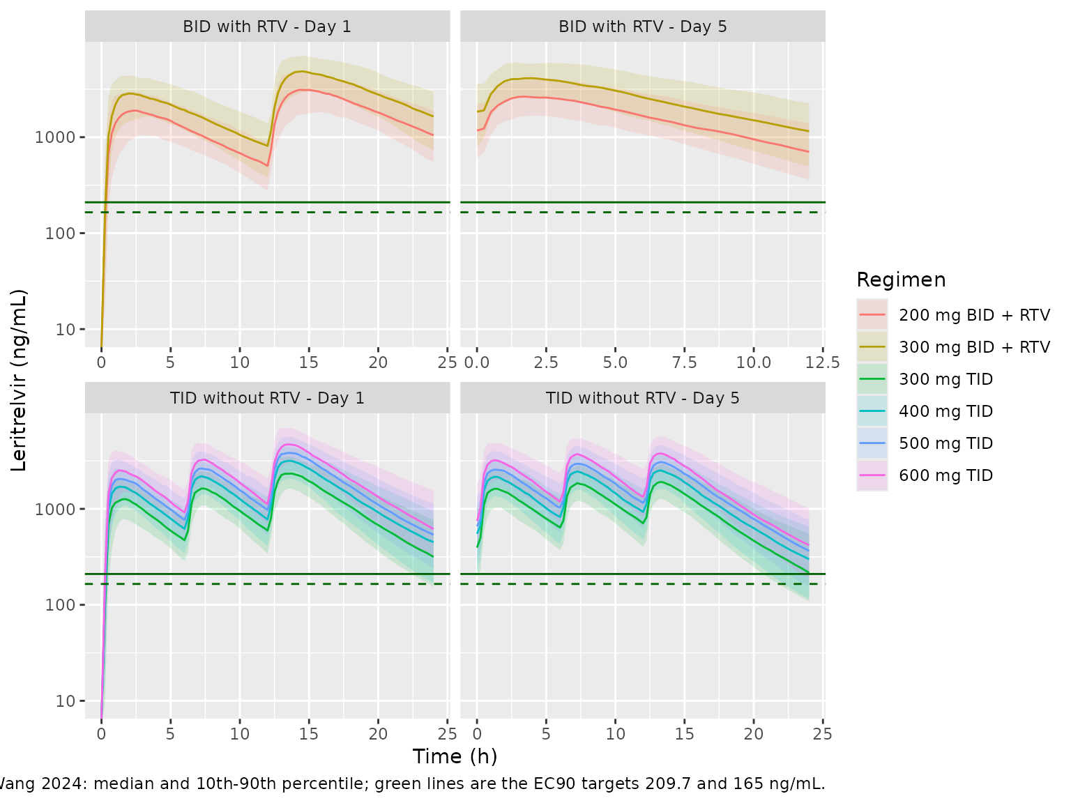
Exposure comparison against Supplementary Table S2 (PKNCA)
Supplementary Table S2 gives geometric-mean exposures for 400 mg TID alone and 300 mg + ritonavir BID in fasted subjects, simulated by the authors from the individual (post hoc) parameters of the 42 and 36 fasted study subjects. The virtual cohort below (100 male and 100 female, full model including the occasion random effects) is a different population, so exact agreement is not expected; the geometric means nevertheless agree closely.
Units are converted to the paper’s: Table S2 reports AUC per day in ngday/mL. For day 1 the interval is 0-24 h, so AUC(0-24) = 24 AUC1. On day 5 the TID interval is 96-120 h (three doses). The BID arm takes its last dose at 96 h, and Table S2’s Cmin,ss (1047 ng/mL) is the Table S1 9th-dose trough at 108 h, so the BID steady-state interval is the 96-108 h dosing interval and AUC(tau) = 12 * AUCss. Cmin is the concentration at the end of each interval, which is how Table S2’s values line up with the Table S1 troughs.
s2_subj <- subjects |>
  filter(Regimen %in% c("400 mg TID", "300 mg BID + RTV"))
ev_s2 <- ev_s1 |> filter(id %in% s2_subj$id)
rxode2::rxSetSeed(20240912)
sim_s2 <- rxode2::rxSolve(ui, ev_s2, returnType = "data.frame", addDosing = FALSE) |>
  left_join(select(subjects, id, Regimen), by = "id")

nca_conc <- bind_rows(
  sim_s2 |> filter(time <= 24) |> mutate(Interval = "Day 1", tint = time),
  sim_s2 |>
    filter(time >= 96, time <= ifelse(grepl("BID", Regimen), 108, 120)) |>
    mutate(Interval = "Day 5", tint = time - 96)
) |>
  filter(!is.na(Cc)) |>
  select(id, Regimen, Interval, tint, Cc)
nca_dose <- ev_s2 |>
  filter(evid == 1L, time %in% c(0, 96)) |>
  left_join(select(subjects, id, Regimen), by = "id") |>
  mutate(Interval = ifelse(time == 0, "Day 1", "Day 5"), tint = 0) |>
  select(id, Regimen, Interval, tint, amt)
nca_int <- tibble(
  Regimen = c("400 mg TID", "400 mg TID", "300 mg BID + RTV", "300 mg BID + RTV"),
  Interval = c("Day 1", "Day 5", "Day 1", "Day 5"),
  start = 0,
  end = c(24, 24, 24, 12),
  cmax = TRUE, auclast = TRUE, clast.obs = TRUE
)
nca_s2 <- PKNCA::pk.nca(PKNCA::PKNCAdata(
  PKNCA::PKNCAconc(nca_conc, Cc ~ tint | Regimen + Interval + id),
  PKNCA::PKNCAdose(nca_dose, amt ~ tint | Regimen + Interval + id),
  intervals = as.data.frame(nca_int)
))

sim_gm <- as.data.frame(nca_s2$result) |>
  filter(PPTESTCD %in% c("cmax", "auclast", "clast.obs")) |>
  group_by(Regimen, Interval, PPTESTCD) |>
  summarise(PPORRES = exp(mean(log(PPORRES))), .groups = "drop")

ref_s2 <- tribble(
  ~Regimen,           ~Interval, ~cmax, ~auclast,     ~clast.obs,
  "400 mg TID",       "Day 1",   3255,  1417 * 24,    413,
  "400 mg TID",       "Day 5",   2565,  1321 * 24,    275,
  "300 mg BID + RTV", "Day 1",   5597,  2739 * 24,   1639,
  "300 mg BID + RTV", "Day 5",   4366,  2592 * 12,   1047
)

s2_tab <- nlmixr2lib::ncaComparisonTable(
  simulated = sim_gm,
  reference = ref_s2,
  by = c("Regimen", "Interval"),
  units = c(cmax = "ng/mL", auclast = "ng*h/mL", clast.obs = "ng/mL")
)
knitr::kable(s2_tab, digits = 0,
caption = "Geometric means: Wang 2024 Supplementary Table S2 (fasted) vs simulation.")| NCA parameter | Regimen | Interval | Reference | Simulated | % diff |
|---|---|---|---|---|---|
| Cmax (ng/mL) | 400 mg TID | Day 1 | 3260 | 3230 | -0.7% |
| Cmax (ng/mL) | 400 mg TID | Day 5 | 2560 | 2590 | +1.1% |
| Cmax (ng/mL) | 300 mg BID + RTV | Day 1 | 5600 | 5020 | -10.2% |
| Cmax (ng/mL) | 300 mg BID + RTV | Day 5 | 4370 | 4280 | -1.9% |
| Clast (ng/mL) | 400 mg TID | Day 1 | 413 | 423 | +2.4% |
| Clast (ng/mL) | 400 mg TID | Day 5 | 275 | 306 | +11.1% |
| Clast (ng/mL) | 300 mg BID + RTV | Day 1 | 1640 | 1610 | -1.5% |
| Clast (ng/mL) | 300 mg BID + RTV | Day 5 | 1050 | 1180 | +12.8% |
| AUClast (ng*h/mL) | 400 mg TID | Day 1 | 34000 | 33800 | -0.6% |
| AUClast (ng*h/mL) | 400 mg TID | Day 5 | 31700 | 32900 | +3.7% |
| AUClast (ng*h/mL) | 300 mg BID + RTV | Day 1 | 65700 | 60600 | -7.9% |
| AUClast (ng*h/mL) | 300 mg BID + RTV | Day 5 | 31100 | 31700 | +1.8% |
attr(s2_tab, "footnote")
#> NULL
s2_pct <- sim_gm |>
  inner_join(
    ref_s2 |> pivot_longer(c(cmax, auclast, clast.obs), names_to = "PPTESTCD", values_to = "ref"),
    by = c("Regimen", "Interval", "PPTESTCD")
  ) |>
  mutate(pct = 100 * (PPORRES / ref - 1))
stopifnot(nrow(s2_pct) == 12)
stopifnot(
  abs(median(s2_pct$pct)) < 8,
  # Realised max |diff| 12.8% at the authoring seed; a cohort-level
  # transcription error in CL, F or Vc moves these by tens of percent.
  quantile(abs(s2_pct$pct), 0.9) < 22
)
Food and sex effects
Supplementary Tables S2 and S3 report the fed-vs-fasted and female-vs-male differences between different groups of study subjects, so subject-to-subject differences are mixed into those percentages. The model’s own effects are simpler. Food multiplies F1 by exp(0.409) = 1.51, so with linear kinetics a fed dose has 51% more AUC than the same subject fasted; the closed-form AUC check above confirms this for the typical subject. Food also multiplies ka by 1.34 and the zero-order duration by 23.2, which moves the peak but not the amount absorbed. The paper’s simulated fed-vs-fasted differences (Table S2: +25 to +63% alone, +29 to +34% with ritonavir) include differences between the fed and fasted study subjects as well.
In the model, female sex lowers CL/F by a factor of exp(-0.224) = 0.80, which raises typical exposure by 25% for both regimens. The paper’s simulated between-group differences (Table S3) are 12-17% without ritonavir and 33-51% with ritonavir; those come from the post hoc parameters of the study subjects and are not a clean read of the covariate effect.
Assumptions and deviations
-
Food-effect rows in Table 2 are transposed. Table 2
lists
Ka.FED = 23.2andD1.FED = 1.34, but the printed Results equations giveKa = 0.293 * exp(0.291 * FED)(exp(0.291) = 1.34) andD1 = 0.0722 * exp(3.14 * FED)(exp(3.14) = 23.1), and the control stream puts THETA(16) on D1 and THETA(17) on Ka. Table 2’s rows follow THETA order with the labels swapped. The model follows the equations and the control stream: food multiplies ka by 1.34 and the zero-order duration by 23.2. -
Occasion variances for the 96 h occasion. Table 2
leaves the OC2.CL and OC2.Vc rows blank, while the equations and the
control stream include
OC2 * eta_OC2on both CL and Vc. A blank row with no estimate is how a NONMEM$OMEGA ... SAMEblock usually appears in a results table, so the OC2 variances are set equal to the OC1 values (19.3% on CL, 54.4% on Vc). As in the control stream, OC1 stays switched on after 96 h, so from 96 h both the OC1 and OC2 terms apply. - IIV scale. Table 2 reports IIV and occasion variability in percent. The 95% confidence intervals are symmetric on the variance scale when the percentage is read as 100 * omega (CL 30.6 [23.6-36.2]: (23.6^2 + 36.2^2) / 2 = 933.7 = 30.6^2 to rounding; D1 155 [106-192] likewise), and not when it is read as a CV with omega^2 = log(1 + CV^2) (for D1 that reading puts the midpoint at a CV of 179%). Variances are therefore (percent / 100)^2.
- Random effects in the control stream but not reported. The control stream carries ETA(4) on Q and ETA(7) on F1, but Table 2, the shrinkage footnote and the printed equations include neither. They are taken as fixed to zero and omitted.
-
Occasion indicators need a multiple-dose flag. The
control stream gates OC1 and OC2 on
DOSESCH > 1and NONMEMTIME(time since the first dose). The model usesMULTI_DOSEfor that flag and rxode2’st, so an event table must start at the first dose of the regimen and single-dose subjects must carryMULTI_DOSE = 0. -
Sex coding. The SEX coding is not printed. The
paper reports higher exposure in females and the CL coefficient is
negative, so SEX = 1 is female, i.e.
SEXF. -
Residual error. The fed-absorption proportional
error (70.2%) applies within 2 h of a fed dose
(
tad() <= 2), as in the control stream. The NONMEM floorIPRED = 0.005for non-positive predictions is not carried over. - Table S1 replication. The occasion random effects are set to zero to match the published simulation (see above), and each arm has 200 subjects rather than 1000.