Clonazepam (Kruizinga 2022) • nlmixr2lib

Model and source

Citation: Kruizinga MD, Zuiker RGJA, Bergmann KR, Egas AC, Cohen AF, Santen GWE, van Esdonk MJ. Population pharmacokinetics of clonazepam in saliva and plasma: Steps towards noninvasive pharmacokinetic studies in vulnerable populations. Br J Clin Pharmacol. 2022;88(5):2236-2245. doi:10.1111/bcp.15152
Description: Two-compartment oral population PK model for clonazepam in plasma and saliva in healthy adults aged 18-30 years given a single 0.5 or 1.0 mg oral solution (Kruizinga 2022). First-order absorption with a two-class mixture on the absorption rate constant: 75% of subjects absorb slowly (ka = 1.106 1/h with IIV) and 25% fast (ka fixed to 100 1/h), encoded by the binary covariate MIX_FAST_ABS. Clearance and inter-compartmental clearance scale allometrically with weight (exponent 0.75) and both volumes linearly, referenced to 70 kg. IIV is carried on the slow-class ka, Q and the relative bioavailability (F fixed to 1). The saliva concentration is the sum of an oral-contamination term and a plasma-driven term. The contamination term is a 1 mL saliva compartment that receives a fraction (0.033 per mille) of the dose and empties first-order (kel_saliva = 1.95 1/h). The plasma-driven term is Cc times a saliva:plasma ratio that rises with plasma concentration by a saturable function (maximum 0.195, half-saturation 2.581 ug/L). A dose must therefore be given TWICE in the event table: once to depot and once, with the same amount, to saliva; the model applies the deposited fraction to the saliva dose through f(saliva).
Article: https://doi.org/10.1111/bcp.15152 (open access; PMC9299763)

Kruizinga 2022 fits a joint plasma + saliva population PK model for clonazepam in healthy young adults, as a step towards a clinical trial in children with ARID1B-related intellectual disability in which blood sampling would be too burdensome. The model is then used to show by simulation that a plasma trough concentration can be predicted from one to five saliva samples by Bayesian MAP estimation.

Population

Twenty healthy subjects aged 18-30 years (mean 22.4, SD 2.8) took part at the Centre for Human Drug Research, Leiden, the Netherlands, in June-July 2020 (Kruizinga 2022 Methods 2.1-2.2 and Table 1). Nine were male (45%), all were Caucasian, and mean (SD) weight was 67.8 (8.3) kg, height 175.1 (7.3) cm and BMI 22.2 (2.4) kg/m^2. Each subject took a single oral dose of 0.5 mg (n = 10) or 1.0 mg (n = 10) clonazepam solution (Rivotril drops) in lemonade. Paired plasma and saliva samples were taken at 0.5, 1, 2, 4, 6, 8, 24 and 48 h; mouths were rinsed with water 10 minutes before each saliva sample, which was collected with a SalivaBio Infant Swab. All 160 plasma samples and 154 of the 160 saliva samples were analysable, and none was below the limit of quantification.

The same information is available programmatically from the model’s population metadata:

pop <- rxode2::rxode(readModelDb("Kruizinga_2022_clonazepam"))$population
#> ℹ parameter labels from comments will be replaced by 'label()'
str(pop, max.level = 1)
#> List of 11
#>  $ species       : chr "human"
#>  $ n_subjects    : num 20
#>  $ n_studies     : num 1
#>  $ age_range     : chr "18-30 years (mean 22.4, SD 2.8)"
#>  $ weight_range  : chr "mean 67.8 kg (SD 8.3)"
#>  $ sex_female_pct: num 55
#>  $ race_ethnicity: Named num 100
#>   ..- attr(*, "names")= chr "Caucasian"
#>  $ disease_state : chr "Healthy volunteers"
#>  $ dose_range    : chr "Single oral dose of 0.5 mg (n = 10) or 1.0 mg (n = 10) clonazepam solution (Rivotril) in lemonade"
#>  $ regions       : chr "Netherlands (Centre for Human Drug Research, Leiden)"
#>  $ notes         : chr "Kruizinga 2022 Methods 2.2 and Table 1: 9 of 20 male, height 175.1 (7.3) cm, BMI 22.2 (2.4) kg/m^2. Paired plas"| __truncated__

Model structure

Plasma. Two-compartment disposition with first-order absorption from a depot. Allometric scaling is fixed and referenced to 70 kg: exponent 0.75 on clearance and intercompartmental clearance, 1 on both volumes. The relative bioavailability is fixed to 1 with between-subject variability (F plasma). The between-subject variance on ka was 0.66 and bimodal, so the authors added a two-class mixture on ka. The fast class has ka fixed at 100 1/h and no variability. The slow class (estimated probability 0.75) has ka = 1.106 1/h with variability. In the packaged model the class is the binary covariate MIX_FAST_ABS (1 = fast class), drawn per subject as Bernoulli(0.25) for a population simulation.

Saliva. The oral solution leaves a residue in the mouth that dominates the saliva concentration for the first ~4 h. The paper models it with a 1 mL contamination compartment. It receives a fraction F saliva of the dose, 0.033 per mille, and empties first-order (Equation 1). After that the saliva concentration is the plasma concentration times a saliva:plasma ratio that rises with plasma concentration towards a ceiling (Equations 2-3):

$\text{ratio} = \text{Ratio}_{MAX} \cdot \frac{C_p}{C_p + \text{Ratio}_{KM}}, \qquad C_{saliva} = \frac{\text{Contamination}}{0.001\,\text{L}} + C_p \cdot \text{ratio}$

The packaged model uses the canonical saliva compartment for the contamination term, with fcontam_saliva, kel_saliva and the fixed volume vsaliva = 0.001 L. The saturable ratio is fsaliva, computed from fsaliva_max and km_fsaliva.

Dosing the contamination compartment. The contamination compartment is not connected to central, so the residue is put in by dosing it directly. Every dose therefore appears twice in the event table: once to depot and once, with the same amount, to saliva. The model applies f(saliva) <- fcontam_saliva, so the saliva record delivers only the residue fraction. The residue is a measurement artefact: it never reaches central and does not reduce the systemic dose.

Source trace

Every ini() value carries an in-file comment pointing to its source. The table below collects them.

Equation / parameter	Value	Source location
`lka` (slow class)	log(1.106) 1/h	Table 2, ‘ka - slow group’
`lka_fastabs` (fast class)	fixed(log(100)) 1/h	Results 3.1 (‘fixed ka of 100/h’)
`MIX_FAST_ABS` probability	0.25 (= 1 - 0.75)	Table 2, ‘Prob. slow group’ = 0.75
`lcl`	log(2.98) L/h	Table 2, ‘clearance’
`lvc`	log(109.5) L	Table 2, ‘VD central’
`lq`	log(61.37) L/h	Table 2, ‘Q’
`lvp`	log(130.6) L	Table 2, ‘VD peripheral’
`lfdepot`	fixed(log(1))	Methods 2.4 (no bioavailability estimable from oral-only data)
`e_wt_cl` (CL, Q)	fixed(0.75)	Methods 2.4; Table 2 footnote
`e_wt_vc` (Vc, Vp)	fixed(1)	Methods 2.4; Table 2 footnote
`lfcontam_saliva`	log(0.033e-3)	Table 2, ‘F saliva’ = 0.033 (% 1000^-1, per mille)
`lkel_saliva`	log(1.95) 1/h	Table 2, ‘Kel saliva’; Equation 1
`lvsaliva`	fixed(log(0.001)) L	Results 3.1 (1 mL fixed); Equation 3
`lfsaliva_max`	log(0.195)	Table 2, ‘RatioMAX’; Equation 2
`lkm_fsaliva`	log(2.581) ug/L	Table 2, ‘RatioKM’; Equation 2
`etalka`	0.16	Table 2, ‘omega2 ka - slow group’
`etalq`	0.25	Table 2, ‘omega2 Q’
`etalfdepot`	0.026	Table 2, ‘omega2 F plasma’
`etalfcontam_saliva`	0.28	Table 2, ‘omega2 F saliva’
`etalkel_saliva`	0.056	Table 2, ‘omega2 Kel saliva’
`propSd` (plasma)	sqrt(0.0058) = 0.0762	Table 2, ‘sigma2 proportional plasma’ (variance)
`propSd_Csaliva`	sqrt(0.057) = 0.239	Table 2, ‘sigma2 proportional saliva’ (variance)
`d/dt(saliva)`	n/a	Equation 1
`fsaliva`	n/a	Equation 2; Table 2 footnote ‘TVRatio’
`Csaliva`	n/a	Equation 3

The Table 2 note states that omega2 and sigma2 are variances, so the residual standard deviations are their square roots.

Typical-value check against Figure 1

Figure 1 of the paper shows the observed mean (SD) plasma and saliva profiles for each dose group. The maintainers digitised the plotted means from the published figure; the 1 mg saliva panel has no plotted mean at 0.5 h. A typical subject (67.8 kg, the Table 1 mean weight; slow absorption class, the majority phenotype) is solved for each dose.

fig1_obs <- tibble::tribble(
  ~dose_mg, ~time, ~plasma, ~saliva,
  0.5, 0.5, 2.42, 9.70,
  0.5, 1,   2.62, 2.73,
  0.5, 2,   2.69, 0.713,
  0.5, 4,   2.46, 0.303,
  0.5, 6,   2.27, 0.230,
  0.5, 8,   2.14, 0.206,
  0.5, 24,  1.92, 0.138,
  0.5, 48,  1.41, 0.091,
  1.0, 0.5, 4.22, NA,
  1.0, 1,   4.65, 4.20,
  1.0, 2,   4.71, 1.28,
  1.0, 4,   3.80, 0.538,
  1.0, 6,   3.56, 0.391,
  1.0, 8,   3.37, 0.365,
  1.0, 24,  2.78, 0.217,
  1.0, 48,  1.98, 0.158
)

mod <- readModelDb("Kruizinga_2022_clonazepam")
mod_typ <- rxode2::zeroRe(mod)
#> ℹ parameter labels from comments will be replaced by 'label()'

make_single_dose <- function(n, dose_mg, times, id_offset = 0L) {
  subj <- tibble(id = id_offset + seq_len(n), dose_mg = dose_mg)
  doses <- subj |>
    tidyr::crossing(cmt = c("depot", "saliva")) |>
    mutate(time = 0, amt = dose_mg, evid = 1L, dvid = NA_integer_)
  obs <- subj |>
    tidyr::crossing(time = times) |>
    mutate(cmt = "central", amt = NA_real_, evid = 0L, dvid = 1L)
  bind_rows(doses, obs) |>
    arrange(id, time, desc(evid))
}

fig1_times <- c(0.5, 1, 2, 4, 6, 8, 24, 48)
ev_typ <- bind_rows(
  make_single_dose(1, 0.5, fig1_times, id_offset = 0L),
  make_single_dose(1, 1.0, fig1_times, id_offset = 1L)
) |>
  mutate(WT = 67.8, MIX_FAST_ABS = 0L)

sim_typ <- rxode2::rxSolve(
  mod_typ,
  events = ev_typ,
  keep = "dose_mg",
  useLinCmt = FALSE # rxode2's ODE->linCmt conversion breaks the dvid mapping
) |>
  as.data.frame()
#> ℹ omega/sigma items treated as zero: 'etalka', 'etalq', 'etalfdepot', 'etalfcontam_saliva', 'etalkel_saliva'
#> Warning: multi-subject simulation without without 'omega'

cmp_fig1 <- sim_typ |>
  select(dose_mg, time, Cc, Csaliva) |>
  inner_join(fig1_obs, by = c("dose_mg", "time")) |>
  mutate(
    ratio_plasma = Cc / plasma,
    ratio_saliva = Csaliva / saliva
  )

cmp_fig1 |>
  mutate(across(c(Cc, Csaliva, ratio_plasma, ratio_saliva), ~ signif(.x, 3))) |>
  rename(
    "Dose (mg)" = dose_mg,
    "Time (h)" = time,
    "Plasma, typical (ug/L)" = Cc,
    "Plasma, Fig 1 mean (ug/L)" = plasma,
    "Plasma ratio" = ratio_plasma,
    "Saliva, typical (ug/L)" = Csaliva,
    "Saliva, Fig 1 mean (ug/L)" = saliva,
    "Saliva ratio" = ratio_saliva
  ) |>
  knitr::kable(caption = "Typical-value prediction vs digitised Figure 1 means.")

Typical-value prediction vs digitised Figure 1 means.
Dose (mg)	Time (h)	Plasma, typical (ug/L)	Saliva, typical (ug/L)	Plasma, Fig 1 mean (ug/L)	Saliva, Fig 1 mean (ug/L)	Plasma ratio	Saliva ratio
0.5	0.5	1.73	6.360	2.42	9.700	0.715	0.656
0.5	1.0	2.37	2.570	2.62	2.730	0.906	0.941
0.5	2.0	2.50	0.574	2.69	0.713	0.929	0.805
0.5	4.0	2.14	0.196	2.46	0.303	0.870	0.647
0.5	6.0	1.99	0.168	2.27	0.230	0.875	0.733
0.5	8.0	1.92	0.159	2.14	0.206	0.896	0.774
0.5	24.0	1.57	0.116	1.92	0.138	0.818	0.840
0.5	48.0	1.17	0.071	1.41	0.091	0.829	0.780
1.0	0.5	3.46	12.800	4.22	NA	0.820	NA
1.0	1.0	4.75	5.290	4.65	4.200	1.020	1.260
1.0	2.0	5.00	1.310	4.71	1.280	1.060	1.020
1.0	4.0	4.28	0.534	3.80	0.538	1.130	0.993
1.0	6.0	3.97	0.470	3.56	0.391	1.120	1.200
1.0	8.0	3.83	0.447	3.37	0.365	1.140	1.220
1.0	24.0	3.14	0.336	2.78	0.217	1.130	1.550
1.0	48.0	2.34	0.217	1.98	0.158	1.180	1.370

The observed data are not dose-proportional. The 48 h dose-normalised plasma mean is 2.8 ug/L per mg in the 0.5 mg group and 2.0 ug/L per mg in the 1 mg group. A linear model fitted to both groups therefore runs about 15% below the 0.5 mg means and about 15% above the 1 mg means. The same split carries through to saliva, amplified by the saturable ratio. Pooled across the two groups, the post-absorption phase agrees closely. The gate below checks that pooled agreement. Plasma is checked from 4 h. Saliva is checked from 6 h, because before then the contamination term dominates.

late_plasma <- cmp_fig1 |> filter(time >= 4)
late_saliva <- cmp_fig1 |> filter(time >= 6, !is.na(saliva))
gm <- function(x) exp(mean(log(x)))
gm_plasma <- gm(late_plasma$ratio_plasma)
gm_saliva <- gm(late_saliva$ratio_saliva)
c(gm_plasma = gm_plasma, gm_saliva = gm_saliva)
#> gm_plasma gm_saliva 
#> 0.9874826 1.0187429

# Deterministic (typical-value) solve against digitised means: a mis-scaled
# CL, V, dose or unit moves every ratio together and breaks the pooled
# geometric mean; the per-point envelope allows for the dose-group imbalance
# described above (pooled plasma GM 0.98, per-point 0.82-1.18; saliva GM
# 1.02, per-point 0.73-1.55 at the time of writing).
stopifnot(
  abs(log(gm_plasma)) < log(1.15),
  all(late_plasma$ratio_plasma > 0.7 & late_plasma$ratio_plasma < 1.4),
  abs(log(gm_saliva)) < log(1.25),
  all(late_saliva$ratio_saliva > 0.5 & late_saliva$ratio_saliva < 2)
)

Virtual cohort for the study design

A stochastic version of the study design: 100 virtual subjects per dose group. Weight is drawn from a normal distribution matching Table 1 (67.8, SD 8.3 kg). Absorption class is drawn as Bernoulli(0.25) for the fast class.

rxode2::rxSetSeed(20220601)
set.seed(20220601)

n_arm <- 100
fine_times <- sort(unique(c(seq(0.25, 8, by = 0.25), seq(9, 48, by = 1))))
ev_study <- bind_rows(
  make_single_dose(n_arm, 0.5, fine_times, id_offset = 0L),
  make_single_dose(n_arm, 1.0, fine_times, id_offset = n_arm)
)
stopifnot(!anyDuplicated(unique(ev_study[, c("id", "time", "evid", "cmt")])))

subj_cov <- tibble(
  id = seq_len(2 * n_arm),
  WT = pmin(pmax(rnorm(2 * n_arm, 67.8, 8.3), 45), 95),
  MIX_FAST_ABS = rbinom(2 * n_arm, 1, 0.25)
)
ev_study <- ev_study |>
  left_join(subj_cov, by = "id") |>
  mutate(treatment = paste(dose_mg, "mg"))

sim_study <- rxode2::rxSolve(
  mod,
  events = ev_study,
  keep = c("treatment", "dose_mg", "WT", "MIX_FAST_ABS"),
  useLinCmt = FALSE
) |>
  as.data.frame()
#> ℹ parameter labels from comments will be replaced by 'label()'

Figure 1 – simulated profiles with the observed means

vpc <- sim_study |>
  select(treatment, time, Plasma = Cc, Saliva = Csaliva) |>
  pivot_longer(c(Plasma, Saliva), names_to = "matrix", values_to = "conc") |>
  group_by(treatment, matrix, time) |>
  summarise(
    Q10 = quantile(conc, 0.10),
    Q50 = median(conc),
    Q90 = quantile(conc, 0.90),
    .groups = "drop"
  )

obs_long <- fig1_obs |>
  mutate(treatment = paste(dose_mg, "mg")) |>
  select(treatment, time, Plasma = plasma, Saliva = saliva) |>
  pivot_longer(c(Plasma, Saliva), names_to = "matrix", values_to = "conc") |>
  filter(!is.na(conc))

ggplot(vpc, aes(time, Q50)) +
  geom_ribbon(aes(ymin = Q10, ymax = Q90), alpha = 0.25, fill = "steelblue") +
  geom_line(colour = "steelblue4") +
  geom_point(data = obs_long, aes(time, conc), inherit.aes = FALSE) +
  facet_grid(matrix ~ treatment, scales = "free_y") +
  scale_y_log10() +
  labs(
    x = "Time (h)",
    y = "Clonazepam concentration (ug/L)",
    title = "Simulated median and 80% interval vs observed means",
    caption = "Replicates Figure 1 of Kruizinga 2022 (points: digitised observed means)."
  )

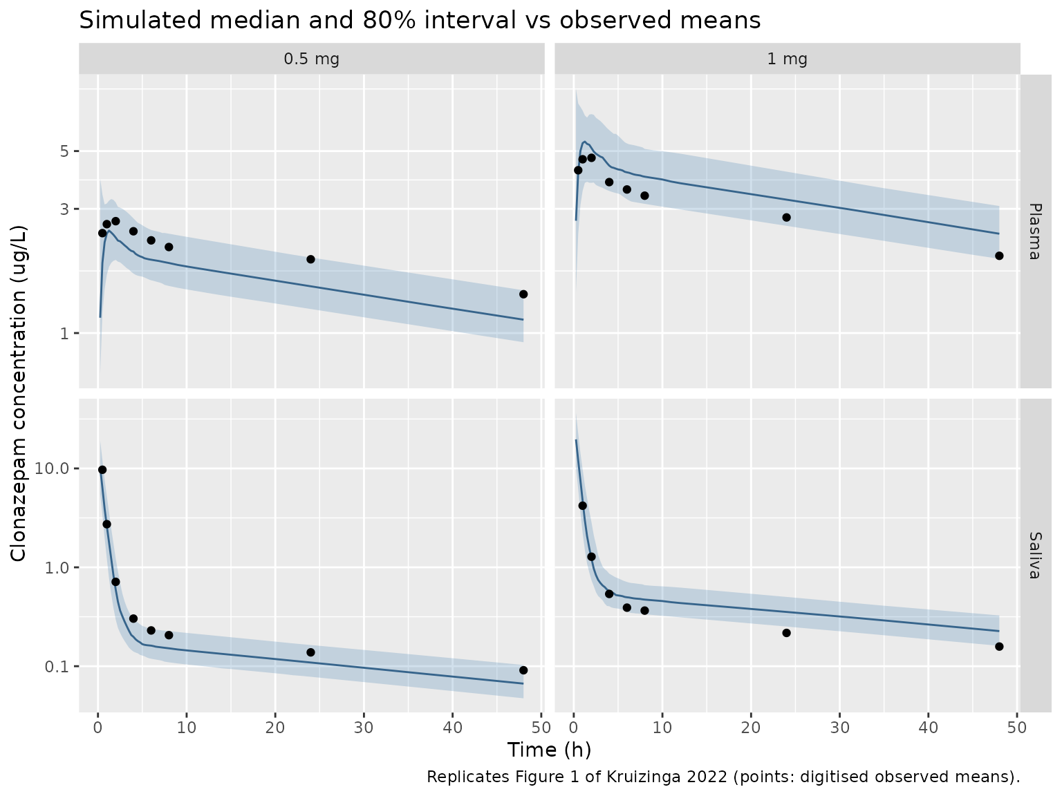
The early saliva peak is the contamination term. It falls with the 1.95 1/h kel_saliva (half-life about 21 minutes). From about 4 h on, saliva tracks plasma through the saturable ratio, as the paper describes.

PKNCA on the study design

The paper reports no NCA, so this table gives the simulated plasma exposures for reference only. The comparison against published values is the trough check in the next section.

nca_conc <- sim_study |>
  filter(!is.na(Cc)) |>
  select(id, time, Cc, treatment)
nca_conc <- bind_rows(
  nca_conc,
  nca_conc |> distinct(id, treatment) |> mutate(time = 0, Cc = 0)
) |>
  distinct(id, treatment, time, .keep_all = TRUE) |>
  arrange(id, treatment, time)

nca_dose <- ev_study |>
  filter(evid == 1, cmt == "depot") |>
  select(id, time, amt, treatment)

conc_obj <- PKNCA::PKNCAconc(
  nca_conc, Cc ~ time | treatment + id,
  concu = "ug/L", timeu = "h"
)
dose_obj <- PKNCA::PKNCAdose(nca_dose, amt ~ time | treatment + id, doseu = "mg")
intervals <- data.frame(
  start = 0, end = 48,
  cmax = TRUE, tmax = TRUE, auclast = TRUE
)
nca_study <- PKNCA::pk.nca(PKNCA::PKNCAdata(conc_obj, dose_obj, intervals = intervals))

as.data.frame(nca_study$result) |>
  group_by(treatment, PPTESTCD) |>
  summarise(median = signif(median(PPORRES), 3), .groups = "drop") |>
  pivot_wider(names_from = PPTESTCD, values_from = median) |>
  rename(
    "Dose group" = treatment,
    "Cmax (ug/L)" = cmax,
    "Tmax (h)" = tmax,
    "AUC0-48 (h*ug/L)" = auclast
  ) |>
  knitr::kable(caption = "Simulated plasma NCA (median) for the study design.")

Simulated plasma NCA (median) for the study design.
Dose group	AUC0-48 (h*ug/L)	Cmax (ug/L)	Tmax (h)
0.5 mg	75.4	2.67	1.5
1 mg	158.0	6.07	1.5

Replicating the paper’s simulation (Figure 2A and Table 3)

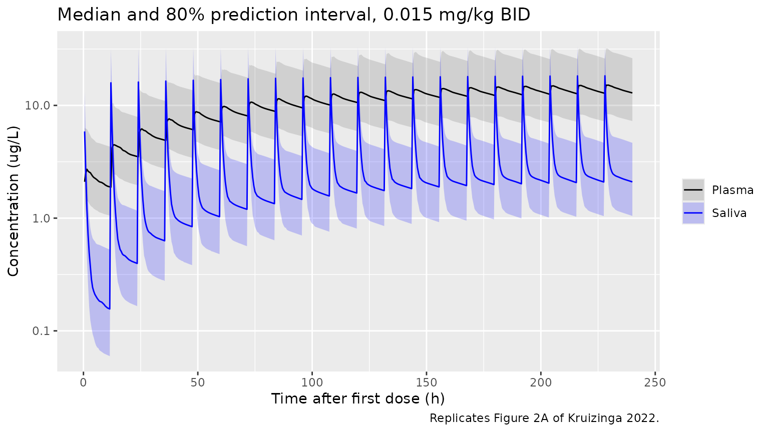
Methods 2.5 describes the paper’s simulation cohort. Age is uniform between 6 and 30 years, with weights between the 10th and 90th centiles for age. Dosing is 0.015 mg/kg twice daily, capped at 0.5 mg per dose. The F plasma variability is raised to a 50% CV, because the healthy-volunteer estimate was thought too narrow for patients. The paper reports a median plasma trough of 2.1 ug/L after dose 1 and 13.7 ug/L at steady state (240 h, after dose 20; Table 3 header). Figure 2A shows the median and 80% prediction interval in plasma and saliva over the 240 h.

The paper does not tabulate the centile curves it used. The cohort below approximates them with a sex-averaged median weight-for-age curve (WHO/CDC style). Each subject’s median is multiplied by a uniform factor between 0.82 and 1.25, an approximate 10th-90th centile band. The cohort is capped at 200 subjects; the paper simulated 2000.

rxode2::rxSetSeed(20220602)
set.seed(20220602)

n_sim <- 200
wt_ref_age <- c(6, 8, 10, 12, 14, 16, 18, 30)
wt_ref_kg <- c(20.5, 25.3, 31.9, 40.0, 49.0, 57.0, 62.0, 72.0)

paper_cohort <- tibble(
  id = seq_len(n_sim),
  AGE = runif(n_sim, 6, 30),
  WT = approx(wt_ref_age, wt_ref_kg, xout = AGE)$y * runif(n_sim, 0.82, 1.25),
  MIX_FAST_ABS = rbinom(n_sim, 1, 0.25)
) |>
  mutate(dose_mg = pmin(0.015 * WT, 0.5))

dose_times <- seq(0, 228, by = 12) # 20 doses; the steady-state trough is at 240 h
obs_times <- seq(0.5, 240, by = 0.5)

ev_paper <- bind_rows(
  paper_cohort |>
    tidyr::crossing(time = dose_times, cmt = c("depot", "saliva")) |>
    mutate(amt = dose_mg, evid = 1L, dvid = NA_integer_),
  paper_cohort |>
    tidyr::crossing(time = obs_times) |>
    mutate(cmt = "central", amt = NA_real_, evid = 0L, dvid = 1L)
) |>
  arrange(id, time, desc(evid)) |>
  mutate(treatment = "0.015 mg/kg BID")

# F plasma CV raised to 50% (Methods 2.5): log-normal variance log(1 + 0.5^2).
mod_paper_sim <- mod |> rxode2::ini(etalfdepot ~ 0.2231436)
#> ℹ parameter labels from comments will be replaced by 'label()'
#> ℹ change initial estimate of `etalfdepot` to `0.2231436`

sim_paper <- rxode2::rxSolve(
  mod_paper_sim,
  events = ev_paper,
  keep = c("treatment", "WT", "AGE"),
  useLinCmt = FALSE
) |>
  as.data.frame()

sim_paper |>
  select(time, Plasma = Cc, Saliva = Csaliva) |>
  pivot_longer(c(Plasma, Saliva), names_to = "matrix", values_to = "conc") |>
  group_by(matrix, time) |>
  summarise(
    Q10 = quantile(conc, 0.10),
    Q50 = median(conc),
    Q90 = quantile(conc, 0.90),
    .groups = "drop"
  ) |>
  ggplot(aes(time, Q50, colour = matrix, fill = matrix)) +
  geom_ribbon(aes(ymin = Q10, ymax = Q90), alpha = 0.2, colour = NA) +
  geom_line() +
  scale_y_log10() +
  scale_colour_manual(values = c(Plasma = "black", Saliva = "blue")) +
  scale_fill_manual(values = c(Plasma = "grey40", Saliva = "blue")) +
  labs(
    x = "Time after first dose (h)",
    y = "Concentration (ug/L)",
    colour = NULL, fill = NULL,
    title = "Median and 80% prediction interval, 0.015 mg/kg BID",
    caption = "Replicates Figure 2A of Kruizinga 2022."
  )

Comparison against published trough medians

PKNCA computes the trough as the last observation in each 12 h interval (clast.obs): after dose 1 over 0-12 h, and at steady state over 228-240 h. The trough uses Cc, the individual prediction without residual error. That matches the paper’s ‘true’ trough, which comes from the simulated individual parameters.

trough_conc <- sim_paper |>
  filter(!is.na(Cc)) |>
  select(id, time, Cc, treatment)
trough_conc <- bind_rows(
  trough_conc,
  trough_conc |> distinct(id, treatment) |> mutate(time = 0, Cc = 0)
) |>
  distinct(id, treatment, time, .keep_all = TRUE) |>
  arrange(id, treatment, time)

trough_dose <- ev_paper |>
  filter(evid == 1, cmt == "depot") |>
  select(id, time, amt, treatment)

trough_intervals <- data.frame(
  start = c(0, 228), end = c(12, 240),
  clast.obs = TRUE
)
nca_trough <- PKNCA::pk.nca(PKNCA::PKNCAdata(
  PKNCA::PKNCAconc(trough_conc, Cc ~ time | treatment + id, concu = "ug/L", timeu = "h"),
  PKNCA::PKNCAdose(trough_dose, amt ~ time | treatment + id, doseu = "mg"),
  intervals = trough_intervals
))

sim_trough <- as.data.frame(nca_trough$result) |>
  mutate(window = ifelse(start == 0, "After dose 1 (12 h)", "Steady state (240 h)")) |>
  select(window, PPTESTCD, PPORRES)

published_trough <- tibble::tribble(
  ~window, ~clast.obs,
  "After dose 1 (12 h)", 2.1,
  "Steady state (240 h)", 13.7
)

cmp_trough <- nlmixr2lib::ncaComparisonTable(
  simulated = sim_trough,
  reference = published_trough,
  by = "window",
  units = c(clast.obs = "ug/L"),
  tolerance_pct = 20
)
knitr::kable(
  cmp_trough,
  caption = "Median plasma trough: simulated vs Kruizinga 2022 Table 3 header."
)

Median plasma trough: simulated vs Kruizinga 2022 Table 3 header.
NCA parameter	window	Reference	Simulated	% diff
Clast (ug/L)	After dose 1 (12 h)	2.1	1.88	-10.4%
Clast (ug/L)	Steady state (240 h)	13.7	12.9	-5.8%

Both medians fall within the 20% tolerance. Most of the remaining difference is Monte-Carlo noise in a 200-subject cohort plus the approximate weight-for-age curve. Across repeated cohorts the simulated medians centre within a few percent of the published 2.1 and 13.7 ug/L.

trough_med <- sim_trough |>
  group_by(window) |>
  summarise(median = median(PPORRES), .groups = "drop") |>
  left_join(published_trough, by = "window") |>
  mutate(pct_diff = 100 * (median - clast.obs) / clast.obs)
trough_med
#> # A tibble: 2 × 4
#>   window               median clast.obs pct_diff
#>   <chr>                 <dbl>     <dbl>    <dbl>
#> 1 After dose 1 (12 h)    1.88       2.1   -10.4 
#> 2 Steady state (240 h)  12.9       13.7    -5.78

# The median of 200 subjects moves with the drawn cohort: over seven seeds it
# ranged from -10% to +11% of the published values (centred near +3%), and the
# seed used here sits at the low end. A mis-scaled CL, volume, F or dose moves
# both medians by tens of percent.
stopifnot(all(abs(trough_med$pct_diff) < 20))

Assumptions and deviations

Figure 1 means are digitised. Kruizinga 2022 does not tabulate the observed concentrations. The maintainers digitised the plotted means from Figure 1 by pixel position against the axis ticks. The 1 mg saliva panel has no plotted mean at 0.5 h.
Absorption mixture as a covariate. The NONMEM mixture is encoded as the binary covariate MIX_FAST_ABS, which the user supplies (1 = fast class, ka fixed at 100 1/h). For a population simulation draw it as Bernoulli(0.25); for a typical-value simulation of the majority phenotype set it to 0. Only the slow class carries etalka, matching Table 2 (‘omega2 ka - slow group’).
Each dose is entered twice. The contamination compartment receives the dose directly, so each dose needs a depot record and a saliva record of the same amount; f(saliva) applies the 0.033 per-mille residue fraction. Leaving out the saliva record removes the early contamination peak but leaves the plasma-driven saliva term (and all plasma predictions) unchanged.
Unit of F saliva. Table 2 prints F saliva as 0.033 in units of ‘% 1000^-1’, which the maintainers read as per mille (3.3e-5 of the dose). With a percent reading (3.3e-4), the 0.5 h saliva prediction would be about 64 ug/L. The plotted means at 0.5 h are below 10 ug/L.
Unit scaling. Dose is in mg and volumes in L, so Cc and Csaliva are multiplied by 1000 to give ug/L, the units of the paper’s figures and of RatioKM.
Simulation cohort. The paper’s weight-for-age centile curves are not given. They are approximated by a sex-averaged median weight-for-age curve times a uniform 0.82-1.25 factor. The cohort has 200 subjects (the paper used 2000). The F plasma variance for this simulation is log(1 + 0.5^2) = 0.223, the log-normal variance for a 50% CV. The paper does not say whether it used this or 0.5^2.
Albumin was tested as a covariate on the saliva:plasma relationship and not retained (Discussion). It is listed in covariatesDataExcluded.
Errata. EuropePMC lists no correction notice linked to Kruizinga 2022 (PMID 34811788) as of 2026-10-08.