Iohexol (Asberg 2020)

Model and source

• Citation: Asberg A, Bjerre A, Almaas R, Luis-Lima S, Robertsen I, Salvador CL, Porrini E, Schwartz GJ, Hartmann A, Bergan S. Measured GFR by Utilizing Population Pharmacokinetic Methods to Determine Iohexol Clearance. Kidney Int Rep. 2020;5(2):189-198. doi:10.1016/j.ekir.2019.11.012. PMC7000849.
• Description: Two-compartment intravenous population PK model for iohexol (Omnipaque 300 mg I/mL) in pediatric and adult patients referred for measured glomerular filtration rate (GFR), developed so that individual iohexol clearance – i.e. measured GFR – can be determined from limited sampling within 5 hours even when GFR is below 40 mL/min. All four structural parameters are scaled allometrically by total body weight standardised to 85 kg (the population median), with exponents fixed at 0.75 on CL and Q and 1 on V and Vp; no other covariate was retained (serum creatinine on CL improved population but worsened individual predictions and was rejected). Estimated with the Pmetrics non-parametric adaptive grid (NPAG) algorithm; the source reports the weighted mean, weighted median and 95% CI of the non-parametric distribution but no parametric between-subject variance, so this is a typical-value model (see the vignette Assumptions and deviations). Residual error is the Pmetrics gamma model on the published HPLC-UV assay SD polynomial. Asberg 2020, development cohort n = 176 patients aged 1-82 years, 1131 serum concentrations.
• Article (open access): https://doi.org/10.1016/j.ekir.2019.11.012
• Supplement (Figures S1-S3): https://europepmc.org/article/PMC/PMC7000849#supplementary-material

Iohexol is a non-ionic X-ray contrast agent that is eliminated almost entirely by glomerular filtration, so its serum clearance is the measured glomerular filtration rate (GFR). The routine clinical method fits a log-linear line through two elimination-phase samples (2 h and 5 h, delayed to 8 h or 24 h when GFR is low) and applies the Brochner-Mortensen correction for the missed distribution phase. Asberg 2020 replaces that with a two-compartment population model used as a Bayesian prior, so that GFR can be read off the individual clearance estimate from four samples within 5 hours (10 min, 30 min, 2 h, 5 h) regardless of renal function.

Population

The development cohort was 176 patients aged 1-82 years (Table 1: 2 aged 0-2 years, 38 aged 2-21, 63 aged 21-60 and 73 over 60), mainly Caucasian and about 76% male, pooled from a prospective Oslo study (2014-2017) and two previously published cohorts from Tenerife and Rochester. Development-cohort mean weight by age bin was 11.4, 45.0, 78.9 and 87.9 kg and mean plasma creatinine 22, 98, 276 and 249 umol/L, i.e. the adult patients were weighted heavily toward reduced renal function. Across development and validation cohorts (219 patients) measured GFR spanned 14-149 mL/min, reported as absolute mL/min rather than per 1.73 m^2.

Each patient received a single IV bolus of 5 mL Omnipaque 300 mg I/mL (3235 mg iohexol; 2 mL in children under 2 years), with the exact dose found by weighing the syringe. The development cohort contributed 1131 serum concentrations (median 7 per patient, range 2-12), measured by HPLC-UV with a lower limit of quantification of 20 mg/L. A validation cohort of 43 patients (395 concentrations) was held out for the limited-sampling evaluation.

Source trace

Model element	Value	Source location
Structure: 2-compartment, IV bolus, parameterised as CL, Q, V, Vp	–	Results, “Model Development” (2-cmt chosen over 1- and 3-cmt)
lcl	log(1.55 L/h) at 85 kg	Table 2, CLs median
lq	log(5.99 L/h) at 85 kg	Table 2, Qs median
lvc	log(10.47 L) at 85 kg	Table 2, Vs median
lvp	log(8.02 L) at 85 kg	Table 2, Vps median
e_wt_cl_q	0.75 (fixed)	Table 2 footnote a; Results final-model equations
e_wt_vc_vp	1 (fixed)	Table 2 footnote a; Results final-model equations
Reference weight	85 kg	Table 2 footnote a; Methods “centralized to population median values”
addSd, propSd, quadSd	0.1523073, 0.01747435, -0.000003919581	Methods, “Model Development” (assay SD polynomial)
gammaSd	1.947	Results, “Model Development” (“The final g value was 1.947”)
Residual model: error = SD * gamma	–	Methods, “Model Development” (gamma error model)
IIV	not encoded	Table 2 reports mean / median / 95% CI only; Figure S1 (see Assumptions)

The typical profile

mod <- rxode2::rxode(readModelDb("Asberg_2020_iohexol"))
dose_std <- 3235 # mg, 5 mL Omnipaque 300 (Methods)

# The typical 85 kg patient, with Table 2 medians.
p <- list(cl = 1.55, q = 5.99, vc = 10.47, vp = 8.02)

The closed-form bi-exponential solution for an IV bolus into the central compartment is the reference for the ODE: both sides use the same parameters, so the difference is pure integration error and a tight bound is correct.

biexp <- function(t, dose, cl, q, vc, vp) {
  k <- cl / vc
  k12 <- q / vc
  k21 <- q / vp
  s <- k + k12 + k21
  alpha <- (s + sqrt(s^2 - 4 * k * k21)) / 2
  beta <- (s - sqrt(s^2 - 4 * k * k21)) / 2
  A <- dose / vc * (alpha - k21) / (alpha - beta)
  B <- dose / vc * (k21 - beta) / (alpha - beta)
  A * exp(-alpha * t) + B * exp(-beta * t)
}

tgrid <- c(0.05, 0.167, 0.5, 1, 2, 3, 5, 8, 12, 24)
ev_typ <- data.frame(
  id = 1L,
  time = c(0, tgrid),
  amt = c(dose_std, rep(0, length(tgrid))),
  evid = c(1L, rep(0L, length(tgrid))),
  cmt = "central",
  WT = 85
)
sim_typ <- rxode2::rxSolve(
  mod, ev_typ,
  rtol = 1e-10, atol = 1e-12, returnType = "data.frame"
)
cf <- biexp(sim_typ$time, dose_std, p$cl, p$q, p$vc, p$vp)
rel_err <- max(abs(sim_typ$Cc / cf - 1))
rel_err
#> [1] 1.81295e-10
# Measured 5e-15 with rxode2 5.1.8 (which still converts to linCmt()); on
# the numeric ODE path (useLinCmt = FALSE) at rtol = 1e-10 it measured
# 1.8e-10. The bound is >100x above the numeric floor so either path passes.
stopifnot(rel_err < 1e-7)

Replicating the supplement’s pcVPC (Figure S2)

Figure S2 is a prediction-corrected VPC of the development cohort. Its red line is the prediction-corrected observed median, which after prediction correction sits on the scale of the median-covariate population prediction – here the 85 kg population-median patient given the standard 3235 mg dose. The line was digitised at its bin vertices from the supplement PDF (axis ticks located from the PDF text layer, red pixels traced at 200 dpi).

Table 2 prints both a weighted mean and a weighted median for every parameter, and they differ 1.7-fold for CL and 1.6-fold for Q, so which column is the typical value is not a formality. Both are overlaid:

fig_s2 <- data.frame(
  time = c(0.27, 1, 2, 3, 4.87, 6, 7, 24),
  Cc_pub = c(276, 191, 149, 126, 98, 98, 93, 28)
)

p_mean <- list(cl = 2.60, q = 9.44, vc = 10.96, vp = 9.44) # Table 2 'Mean'

ev_s2 <- data.frame(
  id = 1L,
  time = c(0, fig_s2$time),
  amt = c(dose_std, rep(0, nrow(fig_s2))),
  evid = c(1L, rep(0L, nrow(fig_s2))),
  cmt = "central",
  WT = 85
)
sim_s2 <- rxode2::rxSolve(mod, ev_s2, returnType = "data.frame")

cmp_s2 <- fig_s2 |>
  mutate(
    Cc_median_params = sim_s2$Cc,
    Cc_mean_params = biexp(time, dose_std, p_mean$cl, p_mean$q, p_mean$vc, p_mean$vp),
    pct_diff_median = 100 * (Cc_median_params / Cc_pub - 1),
    pct_diff_mean = 100 * (Cc_mean_params / Cc_pub - 1)
  )

cmp_s2 |>
  mutate(across(where(is.numeric), \(x) signif(x, 3))) |>
  rename(
    "Time (h)" = time,
    "Figure S2 median (mg/L)" = Cc_pub,
    "Model, Table 2 medians (mg/L)" = Cc_median_params,
    "Table 2 means (mg/L)" = Cc_mean_params,
    "% diff, medians" = pct_diff_median,
    "% diff, means" = pct_diff_mean
  ) |>
  knitr::kable()

Time (h)	Figure S2 median (mg/L)	Model, Table 2 medians (mg/L)	Table 2 means (mg/L)	% diff, medians	% diff, means
0.27	276	258.0	226.00	-6.400	-18.0
1.00	191	183.0	145.00	-4.000	-23.8
2.00	149	144.0	113.00	-3.450	-24.2
3.00	126	126.0	97.90	0.380	-22.3
4.87	98	107.0	78.00	9.300	-20.5
6.00	98	97.8	68.10	-0.243	-30.5
7.00	93	90.2	60.40	-2.960	-35.1
24.00	28	23.3	7.87	-16.900	-71.9

tdense <- seq(0.1, 24, by = 0.1)
curves <- bind_rows(
  data.frame(time = tdense, Cc = biexp(tdense, dose_std, p$cl, p$q, p$vc, p$vp),
             params = "Table 2 medians (encoded)"),
  data.frame(time = tdense, Cc = biexp(tdense, dose_std, p_mean$cl, p_mean$q, p_mean$vc, p_mean$vp),
             params = "Table 2 means")
)
ggplot() +
  geom_line(data = curves, aes(time, Cc, linetype = params)) +
  geom_point(data = fig_s2, aes(time, Cc_pub), colour = "red", size = 2) +
  labs(x = "Time after dose (h)", y = "Iohexol (mg/L)", linetype = NULL) +
  theme_bw() +
  theme(legend.position = "bottom")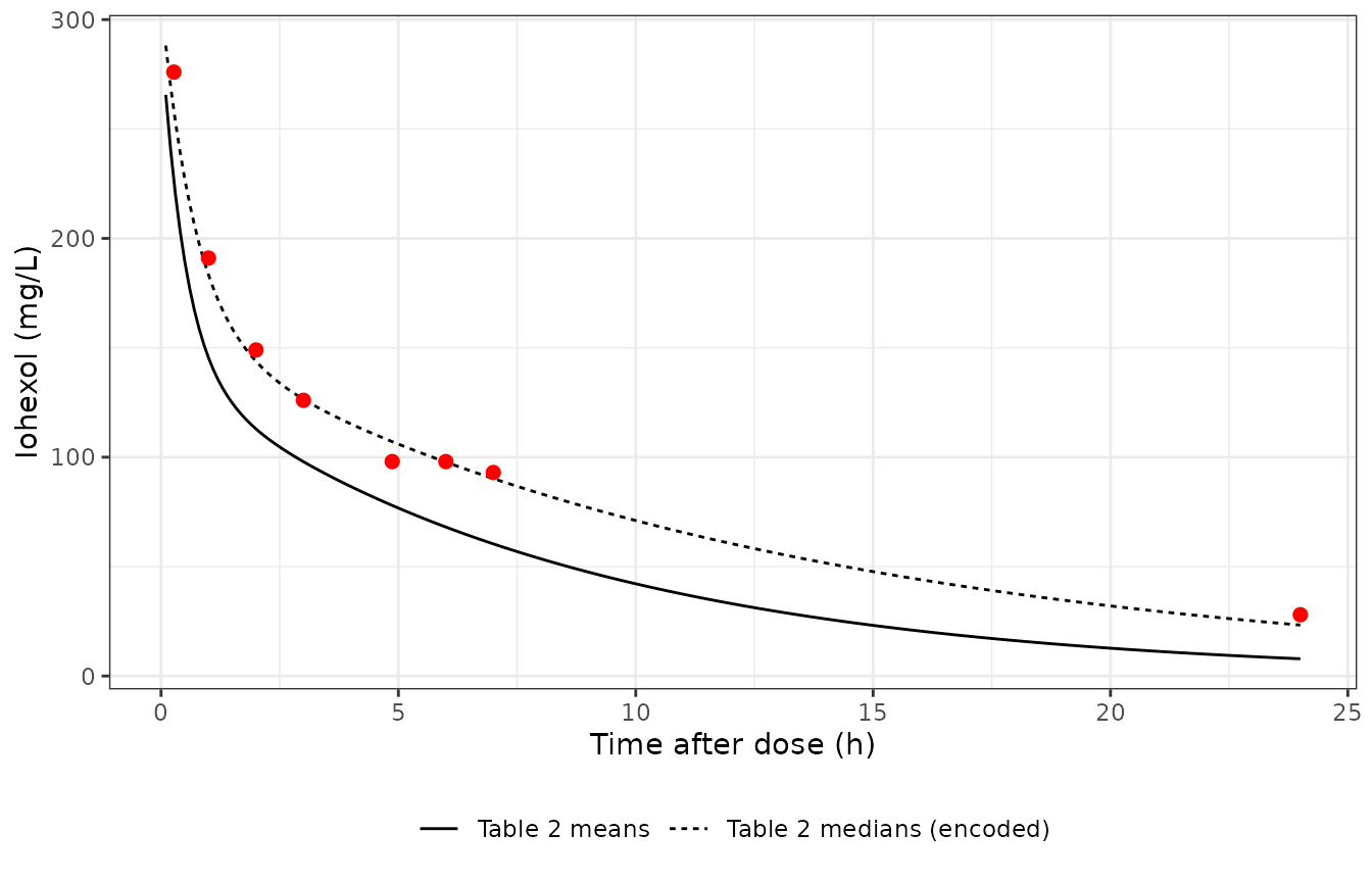

Replicates the observed-median line of Figure S2 of Asberg 2020 (points, digitised). Solid line: this model (Table 2 medians, 85 kg, 3235 mg). Dashed line: the Table 2 means, for contrast.

# The encoded medians track the published median within digitisation and
# binning error (the 24 h bin pools samples drawn over several hours); the
# means undershoot the terminal phase threefold. This is what settles the
# choice of column, and it is deterministic (no simulated cohort).
stopifnot(
  median(abs(cmp_s2$pct_diff_median)) < 10,
  max(abs(cmp_s2$pct_diff_median)) < 25,
  cmp_s2$pct_diff_mean[cmp_s2$time == 24] < -50
)

Body-weight scaling

The only covariate is total body weight, entering all four parameters as (WT/85) with exponents 0.75 on CL and Q and 1 on V and Vp. A small virtual set spanning the development cohort’s age-bin mean weights shows the consequence: the initial concentration scales inversely with weight (volume ~ WT), while the terminal half-life shortens in smaller patients (CL ~ WT^0.75 against V ~ WT).

wts <- c(11.4, 45, 78.9, 87.9) # Table 1 development-cohort age-bin means
doses <- c(3235 * 2 / 5, 3235, 3235, 3235) # 2 mL under 2 years (Methods)
tobs <- c(0, 0.083, 0.167, 0.25, 0.5, 0.75, 1, 1.5, 2, 3, 4, 5, 6, 8, 12, 16, 24, 36, 48)
ev_wt <- bind_rows(lapply(seq_along(wts), function(i) {
  data.frame(
    id = i,
    time = c(0, tobs),
    amt = c(doses[i], rep(0, length(tobs))),
    evid = c(1L, rep(0L, length(tobs))),
    cmt = "central",
    WT = wts[i]
  )
}))
sim_wt <- rxode2::rxSolve(
  mod, ev_wt,
  rtol = 1e-10, atol = 1e-12,
  returnType = "data.frame", keep = "WT"
) |>
  mutate(group = paste0(WT, " kg"))
#> Warning: multi-subject simulation without without 'omega'

ggplot(sim_wt, aes(time, Cc, colour = group)) +
  geom_line() +
  geom_hline(yintercept = 20, linetype = "dotted") +
  scale_y_log10() +
  labs(x = "Time after dose (h)", y = "Iohexol (mg/L, log scale)", colour = "Weight",
       caption = "Dotted line: HPLC-UV LLOQ 20 mg/L") +
  theme_bw()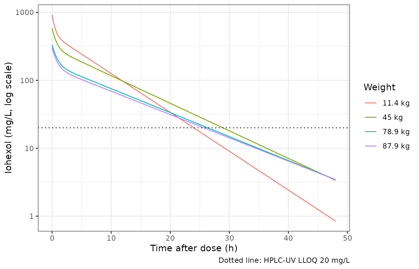

Typical-value iohexol profiles at the Table 1 development-cohort age-bin mean weights (the 11.4 kg child receives the 2 mL dose).

PKNCA validation

Asberg 2020 reports no NCA table, so the NCA check here is whether PKNCA on the typical profiles recovers the clearance (= GFR) and steady-state volume implied by Table 2 after weight scaling – CL = 1.55 (WT/85)^0.75 L/h and Vss = (10.47 + 8.02) (WT/85) L. Profiles run to 48 h and are left uncensored so AUC extrapolation is small.

conc <- sim_wt |>
  filter(!is.na(Cc)) |>
  select(id, time, Cc, group)
dose_df <- ev_wt |>
  filter(evid == 1) |>
  mutate(group = paste0(WT, " kg")) |>
  select(id, time, amt, group)

conc_obj <- PKNCA::PKNCAconc(conc, Cc ~ time | group + id)
dose_obj <- PKNCA::PKNCAdose(dose_df, amt ~ time | group + id, route = "intravascular")
intervals <- data.frame(
  start = 0, end = Inf,
  cl.obs = TRUE, vss.obs = TRUE, aucinf.obs = TRUE, half.life = TRUE, c0 = TRUE
)
nca <- PKNCA::pk.nca(PKNCA::PKNCAdata(conc_obj, dose_obj, intervals = intervals))

reference <- data.frame(
  group = paste0(wts, " kg"),
  cl.obs = 1.55 * (wts / 85)^0.75,
  vss.obs = (10.47 + 8.02) * (wts / 85)
)
tbl <- ncaComparisonTable(
  nca, reference,
  by = "group",
  params = c("cl.obs", "vss.obs"),
  units = c(cl.obs = "L/h", vss.obs = "L")
)
knitr::kable(tbl, caption = "Reference: Table 2 medians scaled by (WT/85)^0.75 (CL) and (WT/85) (Vss).")

Reference: Table 2 medians scaled by (WT/85)^0.75 (CL) and (WT/85) (Vss).

NCA parameter	group	Reference	Simulated	% diff
CL/F (L/h)	11.4 kg	0.344	0.343	-0.1%
CL/F (L/h)	45 kg	0.962	0.961	-0.1%
CL/F (L/h)	78.9 kg	1.47	1.46	-0.1%
CL/F (L/h)	87.9 kg	1.59	1.59	-0.1%
Vss/F (L)	11.4 kg	2.48	2.47	-0.2%
Vss/F (L)	45 kg	9.79	9.77	-0.2%
Vss/F (L)	78.9 kg	17.2	17.1	-0.2%
Vss/F (L)	87.9 kg	19.1	19.1	-0.2%

nca_res <- as.data.frame(nca$result)
cl_nca <- nca_res |> filter(PPTESTCD == "cl.obs") |> arrange(match(group, reference$group))
vss_nca <- nca_res |> filter(PPTESTCD == "vss.obs") |> arrange(match(group, reference$group))
# Linear-up/log-down trapezoids on a 19-point grid; the error is dominated by
# the distribution-phase curvature, measured at < 1% here.
stopifnot(
  max(abs(cl_nca$PPORRES / reference$cl.obs - 1)) < 0.02,
  max(abs(vss_nca$PPORRES / reference$vss.obs - 1)) < 0.05
)

The clinical 2-point method as an independent check

The paper’s comparator, GFR_Clin2, fits a log-linear line through two elimination-phase samples, CL1 = dose / (c1 / b1), and corrects it for the missed distribution phase with GFR_Clin2 = CL1 / (1 + f CL1), f = 0.0032 BSA^-1.3 (Methods; CL1 in mL/min). The second sample is taken at 5 h when eGFR > 40, 8 h when < 40 and 24 h when < 30 mL/min per 1.73 m^2. In the validation cohort GFR_Clin2 agreed with the model-based reference GFR to a relative predictive error of -0.2 +/- 7.1% (Table 3), with 91% of values within 10%.

That agreement is informative about the distribution parameters, which the empirical Brochner-Mortensen correction knows nothing about: if Q, V or Vp were mis-transcribed, the two-point intercept and slope would be biased and the corrected value would drift away from the true clearance. Applying the clinical procedure to noise-free typical-patient profiles, sweeping the true GFR across the paper’s 14-149 mL/min range, is therefore a check that uses a method entirely external to the model. BSA is taken as 2.0 m^2 (Mosteller, 85 kg and 170 cm; Table 1 adult mean heights are 170-179 cm).

gfr_true <- c(15, 20, 25, 30, 35, 40, 50, 60, 80, 100, 120, 150) # mL/min
bsa <- sqrt(170 * 85 / 3600)
t2 <- ifelse(gfr_true < 30, 24, ifelse(gfr_true < 40, 8, 5)) # 85 kg: eGFR/1.73 ~ GFR
ev_c2 <- bind_rows(lapply(seq_along(gfr_true), function(i) {
  data.frame(
    id = i, time = c(0, 2, t2[i]), amt = c(dose_std, 0, 0),
    evid = c(1L, 0L, 0L), cmt = "central", WT = 85
  )
}))
# Per-subject clearance override: the model is typical-value, so lcl is set
# per id through the params table to realise each true GFR.
prm <- data.frame(id = seq_along(gfr_true), lcl = log(gfr_true * 60 / 1000))
sim_c2 <- rxode2::rxSolve(mod, ev_c2, params = prm, returnType = "data.frame")
#> Warning: multi-subject simulation without without 'omega'

clin2 <- sim_c2 |>
  group_by(id) |>
  arrange(time, .by_group = TRUE) |>
  summarise(
    b1 = log(Cc[1] / Cc[2]) / (time[2] - time[1]), # 1/h
    c1 = Cc[1] * exp(b1 * time[1]), # mg/L
    .groups = "drop"
  ) |>
  mutate(
    gfr_true = gfr_true,
    cl1 = dose_std / (c1 / b1) * 1000 / 60, # mL/min
    f = 0.0032 * bsa^-1.3,
    gfr_clin2 = cl1 / (1 + f * cl1),
    pct_diff = 100 * (gfr_clin2 / gfr_true - 1)
  )
clin2 |>
  transmute(
    "True GFR (mL/min)" = gfr_true,
    "Second sample (h)" = t2,
    "CL1, uncorrected (mL/min)" = signif(cl1, 3),
    "GFR_Clin2 (mL/min)" = signif(gfr_clin2, 3),
    "% diff" = signif(pct_diff, 2)
  ) |>
  knitr::kable()

True GFR (mL/min)	Second sample (h)	CL1, uncorrected (mL/min)	GFR_Clin2 (mL/min)	% diff
15	24	15.3	15.0	0.063
20	24	20.3	19.8	-0.970
25	24	25.4	24.6	-1.500
30	8	32.8	31.5	4.900
35	8	38.2	36.4	3.900
40	5	46.5	43.8	9.600
50	5	57.8	53.8	7.500
60	5	69.6	63.8	6.400
80	5	94.8	84.4	5.500
100	5	123.0	106.0	5.700
120	5	153.0	128.0	6.500
150	5	206.0	163.0	8.500

The typical patient sits a few percent above the true GFR (median about +6%, range about -2% to +10%), i.e. inside one standard deviation of the paper’s -0.2 +/- 7.1% and inside its 10% agreement band. A small positive offset at the median distribution parameters is expected: the Table 2 medians of Q and Vp are well below their means, and slower distribution is exactly what makes a two-point line over-read clearance.

The same procedure also reproduces the paper’s motivating problem. If the second sample is always taken at 5 h, the Brochner-Mortensen value drifts upward as GFR falls, because at low GFR a 2-5 h line is still inside the distribution phase – which is why the clinical protocol delays the second sample to 8 or 24 h, and why Asberg 2020 wanted a method that does not.

ev_5h <- ev_c2 |>
  group_by(id) |>
  mutate(time = c(0, 2, 5)) |>
  ungroup()
sim_5h <- rxode2::rxSolve(mod, ev_5h, params = prm, returnType = "data.frame")
#> Warning: multi-subject simulation without without 'omega'
clin2_5h <- sim_5h |>
  group_by(id) |>
  arrange(time, .by_group = TRUE) |>
  summarise(
    b1 = log(Cc[1] / Cc[2]) / (time[2] - time[1]),
    c1 = Cc[1] * exp(b1 * time[1]),
    .groups = "drop"
  ) |>
  mutate(
    gfr_true = gfr_true,
    cl1 = dose_std / (c1 / b1) * 1000 / 60,
    gfr_clin2 = cl1 / (1 + 0.0032 * bsa^-1.3 * cl1),
    pct_diff = 100 * (gfr_clin2 / gfr_true - 1)
  )
clin2_5h |>
  transmute(
    "True GFR (mL/min)" = gfr_true,
    "GFR_Clin2, 2 h + 5 h (mL/min)" = signif(gfr_clin2, 3),
    "% diff" = signif(pct_diff, 2)
  ) |>
  knitr::kable()

True GFR (mL/min)	GFR_Clin2, 2 h + 5 h (mL/min)	% diff
15	19.4	29.0
20	24.3	21.0
25	29.1	16.0
30	34.0	13.0
35	38.9	11.0
40	43.8	9.6
50	53.8	7.5
60	63.8	6.4
80	84.4	5.5
100	106.0	5.7
120	128.0	6.5
150	163.0	8.5

# The paper's own Clin2-vs-reference agreement is -0.2 +/- 7.1% with 91% of
# patients within 10% (Table 3). The typical-patient profiles, sampled per the
# clinical protocol, must sit inside that envelope (measured: median +6.4%,
# max |diff| 9.6%). A mis-read distribution parameter moves the uncorrected
# CL1 by tens of percent and would break this. With the second sample fixed at
# 5 h the error must instead grow as GFR falls (measured +29% at 15 mL/min),
# the paper's stated reason for delayed sampling. Deterministic (no cohort).
stopifnot(
  abs(median(clin2$pct_diff)) < 7.1,
  max(abs(clin2$pct_diff)) < 12,
  clin2_5h$pct_diff[gfr_true == 15] > 20,
  all(diff(clin2_5h$pct_diff[gfr_true <= 40]) < 0)
)

Assumptions and deviations

• Typical values are the Table 2 medians, not the means. Table 2 prints both, weighted by support-point probability, and gives no guidance on which is “typical”. The medians reproduce the supplement’s pcVPC observed median within a few percent across 0.3-24 h, while the means undershoot the 24 h concentration threefold (see above). The medians are also the natural choice for a log-normal-style parameterisation (exp(lcl) is a median).
• No between-subject variability is encoded. NPAG estimates a discrete joint distribution (151 support points), and the paper publishes no SD, CV% or variance. The 95% CI column brackets the mean (CL 2.22-2.97 around 2.60, excluding the median 1.55), so it is precision of the mean, not between-subject spread. Figure S1 shows marginal support-point densities that are flat, bounded and piled up at the search-grid limits (CL 0.2-10 L/h, V 1-20 L, Vp 1-25 L, Q 0-55 L/h), which no log-normal describes. Users who need a stochastic prior can consider two lognormal reconstructions, computed below; they agree for Q but disagree about twofold for V and CL, which is why neither is encoded:

tab2 <- data.frame(
  parameter = c("CL", "Q", "V", "Vp"),
  mean = c(2.60, 9.44, 10.96, 9.44),
  median = c(1.55, 5.99, 10.47, 8.02),
  lo = c(2.22, 8.03, 10.25, 8.66),
  hi = c(2.97, 11.42, 11.68, 10.23)
)
tab2 |>
  mutate(
    omega2_mean_median = 2 * log(mean / median),
    sd_from_ci = (hi - lo) / (2 * 1.96) * sqrt(176),
    omega2_ci = log(1 + (sd_from_ci / mean)^2)
  ) |>
  mutate(across(where(is.numeric), \(x) signif(x, 3))) |>
  rename(
    "Parameter" = parameter,
    "Mean" = mean,
    "Median" = median,
    "95% CI low" = lo,
    "95% CI high" = hi,
    "omega^2 from mean/median" = omega2_mean_median,
    "SD from CI width (n = 176)" = sd_from_ci,
    "omega^2 from CI width" = omega2_ci
  ) |>
  knitr::kable()

Parameter	Mean	Median	95% CI low	95% CI high	omega^2 from mean/median	SD from CI width (n = 176)	omega^2 from CI width
CL	2.60	1.55	2.22	2.97	1.0300	2.54	0.669
Q	9.44	5.99	8.03	11.40	0.9100	11.50	0.907
V	11.00	10.50	10.20	11.70	0.0915	4.84	0.178
Vp	9.44	8.02	8.66	10.20	0.3260	5.31	0.275

• Residual error. The Pmetrics gamma model multiplies the published assay SD polynomial by the fitted gamma (1.947). Pmetrics evaluates that polynomial on the observed concentration; nlmixr2 evaluates it on the prediction (Cc). The quadratic coefficient is negative, so the SD peaks near 2230 mg/L – well above the 20-1100 mg/L validated range and above any concentration a 3235 mg bolus produces in an adult.
• The creatinine covariate model is not encoded. CL = CLs WTc^0.75 exp(CLCRE CREAT) was tested and rejected because it worsened individual predictions; the paper does not print CLCRE.
• Weight range. The development cohort included two children under 2 years; the authors regard the model as validated from 5 to 77 years.
• Limited-sampling results (Table 3) are not reproduced. They are Bayesian posterior estimates in individual patients against the full non-parametric prior, which a typical-value model cannot reproduce.
• The clinical 2-point check assumes BSA 2.0 m^2 and uses the eGFR bands on the true absolute GFR (for an 85 kg, 2.0 m^2 adult, mL/min and mL/min per 1.73 m^2 differ by about 14%, which only moves the 40 and 30 mL/min thresholds, not the correction).