Model and source
- Citation: Gwee A, Duffull S, Zhu X, Tong SYC, Cranswick N, McWhinney B, Ungerer J, Francis J, Steer AC (2020). Population pharmacokinetics of ivermectin for the treatment of scabies in Indigenous Australian children. PLoS Negl Trop Dis 14(12):e0008886. doi:10.1371/journal.pntd.0008886. Parameter values are from the supporting information S1 Text and S1 Table.
- Description: Two-compartment population PK model with first-order absorption for a single oral dose of ivermectin in Indigenous Australian children aged 5 to 15 years and weighing more than 15 kg who were treated for scabies (Gwee 2020, final ‘biological prior’ model). Body weight scales CL/F and Q/F with an exponent fixed to 0.75 and Vc/F and Vp/F with an exponent fixed to 1, all referenced to 37.55 kg; ka is fixed to 0.5 /h. Between-subject variability is a full 4 x 4 block on CL/F, Vc/F, Q/F and Vp/F; the residual error is additive on the log scale.
- Article: PLoS Negl Trop Dis 14(12):e0008886
- Supporting information (S1 Text, S2 Text, S1 Table, S2 Table): https://journals.plos.org/plosntds/article?id=10.1371/journal.pntd.0008886
Gwee et al. fitted two models to the same data and published both in the supporting information:
-
Gwee_2020_ivermectin– the authors’ final model, with the body-weight exponents fixed to their allometric “biological prior” values (0.75 on CL/F and Q/F, 1 on Vc/F and Vp/F). This is the model the paper uses for its dose simulations in children aged 2 to 4 years. -
Gwee_2020_ivermectin_estimatedExponents– the alternative model with the weight exponents on CL/F and Vc/F estimated (0.944 and 2.16) and no weight effect on Q/F or Vp/F. It had the lower objective function value but, in the authors’ words, “provided the same inference in terms of dose prediction”, so it was not carried forward.
Population
The ITCH (Ivermectin Therapy in Children) study enrolled 26 Indigenous Australian children with scabies in a remote community in Arnhem Land, Northern Territory, between April 2016 and March 2018. Eleven (42%) were male; the median age was 10.9 years (range 5.5 to 14.9) and the median body weight 37.6 kg (18.5 to 74.5). Children received a single oral dose of 200 ug/kg rounded to the nearest whole or half 3 mg tablet with food (median 190 ug/kg, range 120 to 230). Each child gave two plasma samples (one child gave one), for 48 concentrations in total, drawn in one of five sampling-design groups that together span 2 hours to 14 days after the dose (Table 1 of the paper). The lower limit of quantification was 2 ug/L. Demographics are from the first paragraph of the Results; the paper has no baseline-characteristics table.
The same information is available programmatically via
readModelDb("Gwee_2020_ivermectin")()$population.
Source trace
The per-parameter origin is recorded as an in-file comment next to
each ini() entry in
inst/modeldb/specificDrugs/Gwee_2020_ivermectin.R and
inst/modeldb/specificDrugs/Gwee_2020_ivermectin_estimatedExponents.R.
| Equation / parameter | Final model | Estimated-exponent model | Source location |
|---|---|---|---|
| Structure: 2 compartments, first-order absorption, linear elimination | – | – | Results, paragraph 2 |
CL/F = TVCL * (WT/37.55)^e_wt_cl |
6.94 L/h, exponent 0.75 fixed | 6.73 L/h, exponent 0.944 | S1 / S2 Text; S1 / S2 Table |
Vc/F = TVVc * (WT/37.55)^e_wt_vc |
88 L, exponent 1 fixed | 160 L, exponent 2.16 | S1 / S2 Text; S1 / S2 Table |
Q/F |
13.7 L/h x (WT/37.55)^0.75 (fixed) | 2.95 L/h, no weight effect | S1 / S2 Text; S1 / S2 Table |
Vp/F |
344 L x (WT/37.55) (fixed) | 447 L, no weight effect | S1 / S2 Text; S1 / S2 Table |
ka |
0.5 1/h fixed | 0.5 1/h fixed | S1 / S2 Table |
| BSV %CV (CL, Vc, Q, Vp) | 54, 237.1, 40.8, 38.9 | 68.7, 86.9, 108.7, 29.8 | S1 / S2 Table, read as described below |
| Correlations (CL-Vc, CL-Q, CL-Vp, Vc-Q, Vc-Vp, Q-Vp) | -0.30, 0.70, 0.863, 0.467, 0.215, 0.964 | -0.042, 0.399, -0.958, -0.934, -0.239, -0.125 | S1 / S2 Table, read as described below |
Residual error, SD of an additive error on the log scale
(Cc ~ lnorm(expSd)) |
0.198 | 0.062 | S1 / S2 Table |
Cc = 1000 * central / vc (mg and L to ug/L) |
– | – | Units: dose in mg, concentrations in ug/L (Methods) |
Reading the variability block of S1 and S2 Tables
Both supporting tables print the between-subject-variability block with the value column one row above its labels. The block has 11 label rows (a heading, four %CV rows and six correlation rows) but only 10 values: the first value sits on the heading row, and the last label, “Correlation (Q, Vp)”, has no value. Read literally, the Vp row would carry a %CV of “-30%”, which is impossible. Read in order, the 10 values are the four %CVs (CL, Vc, Q, Vp) followed by the six correlations in the printed label order, which is how they are encoded here.
The tables do not say whether “%CV” means 100 * omega
(the standard-deviation scale) or the exact log-normal CV,
100 * sqrt(exp(omega^2) - 1). For the Vc/F entry of 237.1%
the two readings give omega^2 = 5.62 or 1.89, so the choice matters. The
maintainers took the SD-scale reading, omega = CV/100, for
two reasons that are both checked below:
- Figure 1 (pcVPC). In the earliest time bin, the model’s 10th percentile is about 4 ug/L. Under the SD-scale reading the packaged model gives about 3.3 ug/L; under the log-normal reading it gives about 10.5 ug/L.
- Simulated AUC spread. For one 3 mg tablet in children weighing 10 to 15 kg the paper reports a median AUC of 976 ug*h/L with an IQR of 671 to 1384. The SD-scale reading reproduces the width of that IQR; the log-normal reading gives an IQR that is too narrow.
Virtual cohorts
The observed data are not public. Two virtual populations are used.
- Study population (children aged 5 to 15 years). Age is uniform from 5.5 to 14.9 years. Weight follows an exponential weight-for-age curve with 10.5% growth per year and a log-normal SD of 0.2, passing through the reported median weight (37.6 kg) at the median age of the virtual cohort (10.2 years), so that the virtual median weight matches the study’s. Weights outside the observed 18.5 to 74.5 kg range are redrawn, not clamped. The dose is 200 ug/kg rounded to the nearest half 3 mg tablet (1.5 mg steps).
- Children aged 2 to 4 years weighing 10 to 15 kg. The paper used a separate covariate database of 288 children that is not published, so weight is taken as uniform from 10 to 15 kg. The same weights are dosed two ways, as in the paper: (i) 200 ug/kg rounded to the nearest half or whole 3 mg tablet (1.5 mg below 11.25 kg, 3 mg above), and (ii) one 3 mg tablet.
rxode2::rxSetSeed(20201207)
set.seed(20201207)
n_arm <- 200

draw_study_weights <- function(age) {
  wt <- 37.6 * exp(0.105 * (age - 10.2) + rnorm(length(age), 0, 0.2))
  bad <- wt < 18.5 | wt > 74.5
  while (any(bad)) {
    wt[bad] <- 37.6 * exp(0.105 * (age[bad] - 10.2) + rnorm(sum(bad), 0, 0.2))
    bad <- wt < 18.5 | wt > 74.5
  }
  wt
}

round_to_half_tablet <- function(dose_mg) {
  pmax(1.5, round(dose_mg / 1.5) * 1.5)
}

age_study <- runif(n_arm, 5.5, 14.9)
wt_study <- draw_study_weights(age_study)
wt_young <- runif(n_arm, 10, 15)

subjects <- dplyr::bind_rows(
  tibble(
    id = seq_len(n_arm), treatment = "Study population, 200 ug/kg rounded",
    AGE = age_study, WT = wt_study, amt = round_to_half_tablet(0.2 * wt_study)
  ),
  tibble(
    id = n_arm + seq_len(n_arm), treatment = "Age 2-4 y, 200 ug/kg rounded",
    AGE = NA_real_, WT = wt_young, amt = round_to_half_tablet(0.2 * wt_young)
  ),
  tibble(
    id = 2 * n_arm + seq_len(n_arm), treatment = "Age 2-4 y, 3 mg",
    AGE = NA_real_, WT = wt_young, amt = 3
  )
)

# Log-spaced grid: the Vc/F variability is large, so the absorption peak must
# be resolved for every subject; 2000 h is more than 30 typical terminal
# half-lives.
obs_times <- c(0, exp(seq(log(0.05), log(2000), length.out = 90)))

events <- dplyr::bind_rows(
  subjects |> dplyr::mutate(time = 0, evid = 1L, cmt = "depot"),
  subjects |>
    dplyr::select(-amt) |>
    tidyr::crossing(time = obs_times) |>
    dplyr::mutate(evid = 0L, amt = 0, cmt = "central")
) |>
  dplyr::arrange(id, time, dplyr::desc(evid))
stopifnot(!anyDuplicated(unique(events[, c("id", "time", "evid")])))

subjects |>
  group_by(treatment) |>
  summarise(
    `Median WT (kg)` = median(WT),
    `WT range (kg)` = sprintf("%.1f-%.1f", min(WT), max(WT)),
    `Median dose (ug/kg)` = median(1000 * amt / WT),
    .groups = "drop"
  ) |>
knitr::kable(digits = 1, caption = "Virtual cohorts.")| treatment | Median WT (kg) | WT range (kg) | Median dose (ug/kg) |
|---|---|---|---|
| Age 2-4 y, 200 ug/kg rounded | 12.4 | 10.1-14.9 | 216.3 |
| Age 2-4 y, 3 mg | 12.4 | 10.1-14.9 | 242.3 |
| Study population, 200 ug/kg rounded | 36.1 | 20.0-72.7 | 199.3 |
Simulation
mod <- readModelDb("Gwee_2020_ivermectin")
sim <- rxode2::rxSolve(
  mod,
  events = events,
  keep = c("treatment", "WT", "AGE"),
  returnType = "data.frame"
)
stopifnot(!anyNA(sim$Cc))
Replicate Figure 1 (prediction-corrected VPC)
A prediction-corrected VPC rescales every observation to the typical prediction of its bin, which removes the effect of dose and body weight. The equivalent simulation gives every virtual subject the median weight (37.55 kg) and the median dose (190 ug/kg x 37.6 kg = 7.14 mg), with between-subject and residual variability. The points are the model percentiles of Figure 1, digitised by the maintainers (approximate; the paper’s percentiles are over time bins spanning 0 to 15 h, 15 to 40 h, 40 to 105 h, 105 to 220 h and 220 to 340 h).
fig1_published <- tibble::tribble(
  ~time, ~p10, ~p50, ~p90,
  3.6, 4.3, 35.2, 50.7,
  25, 3.66, 6.3, 14.3,
  49, 1.70, 3.38, 5.46,
  177, 0.177, 1.12, 4.94,
  283, 0.113, 0.31, 2.68
)

vpc_times <- c(0.5, 1, 2, 3, 3.6, 4, 6, 8, 12, 18, 25, 36, 49, 72, 100, 140, 177, 220, 283, 340)
vpc_events <- tibble(id = seq_len(n_arm), WT = 37.55) |>
  tidyr::crossing(time = c(0, vpc_times)) |>
  dplyr::mutate(
    evid = ifelse(time == 0, 1L, 0L),
    amt = ifelse(time == 0, 7.14, 0),
    cmt = ifelse(time == 0, "depot", "central")
  )
vpc_events <- dplyr::bind_rows(
  vpc_events,
  vpc_events |> dplyr::filter(time == 0) |> dplyr::mutate(evid = 0L, amt = 0, cmt = "central")
) |>
  dplyr::arrange(id, time, dplyr::desc(evid))

vpc_sim <- rxode2::rxSolve(mod, events = vpc_events, returnType = "data.frame") |>
  dplyr::filter(time > 0)

vpc_q <- vpc_sim |>
  group_by(time) |>
  summarise(
    p10 = quantile(sim, 0.10), p50 = quantile(sim, 0.50), p90 = quantile(sim, 0.90),
    .groups = "drop"
  )

ggplot(vpc_q, aes(time)) +
  geom_ribbon(aes(ymin = p10, ymax = p90), alpha = 0.2, fill = "steelblue") +
  geom_line(aes(y = p50), colour = "steelblue") +
  geom_point(
    data = tidyr::pivot_longer(fig1_published, -time, names_to = "pct", values_to = "conc"),
    aes(time, conc, shape = pct), colour = "red"
  ) +
  scale_y_log10() +
  labs(
    x = "Time after dose (h)", y = "Ivermectin (ug/L)", shape = "Figure 1",
    title = "Figure 1 - 10th, 50th and 90th percentiles",
    caption = "Band and line: packaged model. Red points: digitised from Figure 1 of Gwee 2020."
  )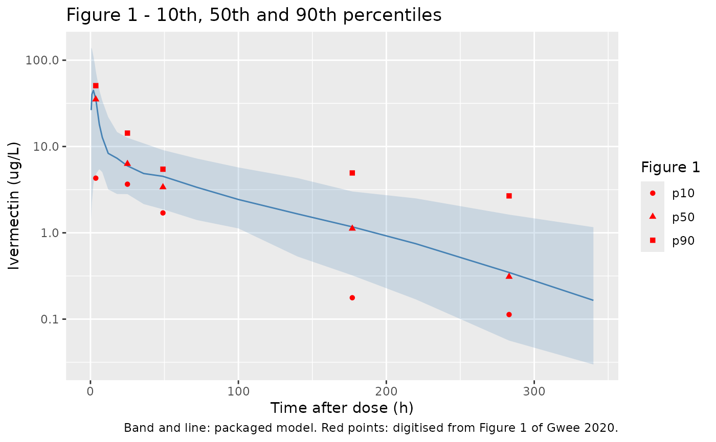
fig1_published |>
  dplyr::inner_join(vpc_q, by = "time", suffix = c("_published", "_model")) |>
  dplyr::select(time, p10_published, p10_model, p50_published, p50_model, p90_published, p90_model) |>
  dplyr::rename(
    "Time (h)" = time,
    "P10 Figure 1" = p10_published, "P10 model" = p10_model,
    "P50 Figure 1" = p50_published, "P50 model" = p50_model,
    "P90 Figure 1" = p90_published, "P90 model" = p90_model
  ) |>
knitr::kable(digits = 2, caption = "Figure 1 percentiles (digitised) vs. the packaged model (ug/L).")| Time (h) | P10 Figure 1 | P10 model | P50 Figure 1 | P50 model | P90 Figure 1 | P90 model |
|---|---|---|---|---|---|---|
| 3.6 | 4.30 | 4.23 | 35.20 | 34.87 | 50.70 | 74.91 |
| 25.0 | 3.66 | 2.81 | 6.30 | 5.97 | 14.30 | 12.64 |
| 49.0 | 1.70 | 1.87 | 3.38 | 4.52 | 5.46 | 9.10 |
| 177.0 | 0.18 | 0.32 | 1.12 | 1.17 | 4.94 | 3.01 |
| 283.0 | 0.11 | 0.06 | 0.31 | 0.35 | 2.68 | 1.63 |
fig1_check <- dplyr::inner_join(fig1_published, vpc_q, by = "time", suffix = c("_pub", "_mod"))
stopifnot(nrow(fig1_check) == 5)
# The median is the structural check: dose, CL/F, Vc/F and the distribution
# phase all set it. Its first-bin value is taken at 3.6 h on a steep rising
# and falling peak, so allow for the bin position.
stopifnot(abs(median(log(fig1_check$p50_mod / fig1_check$p50_pub))) < log(1.3))
The model’s median tracks the published median from the absorption peak to the last bin, within about a third at every bin and more closely at most. The published percentiles are prediction-corrected within wide time bins that each hold roughly 8 to 14 of the 48 observations, so the 10th and 90th percentiles agree only in magnitude; the flat published 90th percentile between 50 and 180 h is a feature of that binning.
Which %CV scale Figure 1 supports
The earliest bin is where the two readings of the %CV column separate. A 10th percentile estimated from 200 random subjects varies by about a factor of two between draws here, because the Vc/F variability is so large. The chunk below therefore uses a fixed, stratified set of 199 random-effect vectors (a rank-1 lattice mapped through the normal quantile function and the Cholesky factor of the omega matrix), so the result is the same on every machine. It solves the typical subject of Figure 1 at 4 h under the packaged omega and under the omega rebuilt with the log-normal reading and the same correlations.
ui <- rxode2::rxode(mod)
omega_sd <- ui$omega
cv <- sqrt(diag(omega_sd))
sd_lognormal <- sqrt(log(1 + cv^2))
omega_lognormal <- diag(sd_lognormal) %*% stats::cov2cor(omega_sd) %*% diag(sd_lognormal)
dimnames(omega_lognormal) <- dimnames(omega_sd)

# Rank-1 lattice: n prime, each coordinate takes every stratum (k + 0.5)/n once.
lattice_etas <- function(omega, n = 199, gen = c(1, 45, 70, 110)) {
  u <- (outer(seq_len(n) - 1, gen) %% n + 0.5) / n
  eta <- stats::qnorm(u) %*% chol(omega)
  colnames(eta) <- colnames(omega)
  as.data.frame(eta)
}

p10_at_4h <- function(omega) {
  etas <- lattice_etas(omega)
  ev <- data.frame(
    id = rep(seq_len(nrow(etas)), each = 2), time = c(0, 4), evid = c(1L, 0L),
    amt = c(7.14, 0), cmt = c("depot", "central"), WT = 37.55
  )
  # The random effects are supplied as parameters, so rxode2's note that a
  # multi-subject solve has no omega is expected here.
  s <- withCallingHandlers(
    rxode2::rxSolve(rxode2::zeroRe(ui), events = ev, params = etas, returnType = "data.frame"),
    warning = function(w) {
      if (grepl("without 'omega'", conditionMessage(w))) invokeRestart("muffleWarning")
    }
  )
  stopifnot(nrow(s) == nrow(etas), !anyNA(s$Cc))
  unname(quantile(s$Cc, 0.10))
}

p10_tab <- tibble(
  Reading = c("Published Figure 1 (first bin)", "SD scale, omega = CV (packaged)", "Log-normal CV"),
  `10th percentile at 4 h (ug/L)` = c(4.3, p10_at_4h(omega_sd), p10_at_4h(omega_lognormal))
)
knitr::kable(p10_tab, digits = 2)| Reading | 10th percentile at 4 h (ug/L) |
|---|---|
| Published Figure 1 (first bin) | 4.30 |
| SD scale, omega = CV (packaged) | 3.32 |
| Log-normal CV | 10.54 |
Typical-value AUC against the paper’s simulations
For a linear model the median AUC of a cohort equals the
typical-subject AUC, 1000 * Dose / CL, at the median
covariate. This is a deterministic check of the clearance, its weight
exponent and the units.
typical_auc <- function(model, dose_mg, wt) {
  ev <- tibble(id = 1L, time = c(0, 1), evid = c(1L, 0L), amt = c(dose_mg, 0),
               cmt = c("depot", "central"), WT = wt)
  s <- rxode2::rxSolve(rxode2::zeroRe(model), events = ev, returnType = "data.frame")
  1000 * dose_mg / s$cl[1]
}

typ_tab <- tibble::tribble(
  ~Scenario, ~dose, ~wt, ~published,
  "Study population: 190 ug/kg at 37.6 kg", 0.190 * 37.6, 37.6, 1001,
  "One 3 mg tablet, 10-15 kg (at 12.5 kg)", 3, 12.5, 976,
  "One 3 mg tablet, 12-15 kg (at 13.5 kg)", 3, 13.5, 953
) |>
  dplyr::rowwise() |>
  dplyr::mutate(model = typical_auc(mod, dose, wt)) |>
  dplyr::ungroup() |>
  dplyr::mutate(pct_diff = 100 * (model / published - 1))
#> ℹ omega/sigma items treated as zero: 'etalcl', 'etalvc', 'etalq', 'etalvp'
#> ℹ omega/sigma items treated as zero: 'etalcl', 'etalvc', 'etalq', 'etalvp'
#> ℹ omega/sigma items treated as zero: 'etalcl', 'etalvc', 'etalq', 'etalvp'

typ_tab |>
  dplyr::rename(
    "Dose (mg)" = dose, "WT (kg)" = wt,
    "Published median AUC (ug*h/L)" = published,
    "Typical-value AUC (ug*h/L)" = model, "% diff" = pct_diff
  ) |>
knitr::kable(digits = 1)| Scenario | Dose (mg) | WT (kg) | Published median AUC (ug*h/L) | Typical-value AUC (ug*h/L) | % diff |
|---|---|---|---|---|---|
| Study population: 190 ug/kg at 37.6 kg | 7.1 | 37.6 | 1001 | 1028.4 | 2.7 |
| One 3 mg tablet, 10-15 kg (at 12.5 kg) | 3.0 | 12.5 | 976 | 986.4 | 1.1 |
| One 3 mg tablet, 12-15 kg (at 13.5 kg) | 3.0 | 13.5 | 953 | 931.0 | -2.3 |
PKNCA validation
sim_nca <- sim |>
  dplyr::filter(!is.na(Cc)) |>
  dplyr::select(id, time, Cc, treatment)
# Numeric-path undershoot in the far tail is integrator noise; floor it.
stopifnot(all(sim_nca$Cc >= -1e-6 * max(sim_nca$Cc)))
sim_nca <- sim_nca |> dplyr::mutate(Cc = pmax(Cc, 0))
sim_nca <- dplyr::bind_rows(
  sim_nca,
  sim_nca |> dplyr::distinct(id, treatment) |> dplyr::mutate(time = 0, Cc = 0)
) |>
  dplyr::distinct(id, treatment, time, .keep_all = TRUE) |>
  dplyr::arrange(id, treatment, time) |>
  dplyr::group_by(id) |>
  dplyr::filter(time <= time[which.max(Cc)] | Cc >= 1e-6 * max(Cc)) |>
  dplyr::ungroup()

dose_df <- events |>
  dplyr::filter(evid == 1) |>
  dplyr::select(id, time, amt, treatment)

conc_obj <- PKNCA::PKNCAconc(sim_nca, Cc ~ time | treatment + id)
dose_obj <- PKNCA::PKNCAdose(dose_df, amt ~ time | treatment + id)
intervals <- data.frame(
  start = 0, end = Inf,
  cmax = TRUE, tmax = TRUE, aucinf.obs = TRUE, half.life = TRUE
)
nca_res <- PKNCA::pk.nca(PKNCA::PKNCAdata(conc_obj, dose_obj, intervals = intervals))

auc_subj <- as.data.frame(nca_res) |>
  dplyr::filter(PPTESTCD == "aucinf.obs") |>
  dplyr::select(id, treatment, aucinf.obs = PPORRES) |>
  dplyr::left_join(
    sim |> dplyr::filter(time == 0) |> dplyr::distinct(id, cl, WT, AGE),
    by = "id"
  ) |>
  dplyr::left_join(dose_df |> dplyr::select(id, amt), by = "id")

# Mass balance: PKNCA AUCinf must equal 1000 * Dose / CL for every subject.
auc_ratio <- auc_subj$aucinf.obs / (1000 * auc_subj$amt / auc_subj$cl)
stopifnot(abs(median(auc_ratio) - 1) < 0.01, quantile(abs(auc_ratio - 1), 0.9) < 0.03)
Comparison against published AUC medians
The paper reports the median AUC for the enrolled children overall and by age group (from individual clearances), and for the simulated children aged 2 to 4 years by dosing strategy and weight band. The weight bands for the young children split at 11.25 kg, the weight at which 200 ug/kg rounds up from 1.5 mg to 3 mg.
sim_groups <- dplyr::bind_rows(
  auc_subj |> dplyr::filter(treatment == "Study population, 200 ug/kg rounded") |>
    dplyr::mutate(group = "Study population, all"),
  auc_subj |> dplyr::filter(treatment == "Study population, 200 ug/kg rounded", AGE <= 11) |>
    dplyr::mutate(group = "Study population, 5-11 y"),
  auc_subj |> dplyr::filter(treatment == "Study population, 200 ug/kg rounded", AGE > 11) |>
    dplyr::mutate(group = "Study population, >11 y"),
  auc_subj |> dplyr::filter(treatment == "Age 2-4 y, 200 ug/kg rounded") |>
    dplyr::mutate(group = "2-4 y, 200 ug/kg rounded, all"),
  auc_subj |> dplyr::filter(treatment == "Age 2-4 y, 200 ug/kg rounded", WT < 11.25) |>
    dplyr::mutate(group = "2-4 y, 200 ug/kg rounded, <11 kg"),
  auc_subj |> dplyr::filter(treatment == "Age 2-4 y, 3 mg") |>
    dplyr::mutate(group = "2-4 y, 3 mg, all"),
  auc_subj |> dplyr::filter(treatment == "Age 2-4 y, 3 mg", WT < 11.25) |>
    dplyr::mutate(group = "2-4 y, 3 mg, 10-11 kg"),
  auc_subj |> dplyr::filter(treatment == "Age 2-4 y, 3 mg", WT >= 11.25) |>
    dplyr::mutate(group = "2-4 y, 3 mg, 12-15 kg")
) |>
  dplyr::group_by(group) |>
  dplyr::summarise(aucinf.obs = median(aucinf.obs), n = dplyr::n(), .groups = "drop")
stopifnot(nrow(sim_groups) == 8, all(sim_groups$n >= 20))

published_auc <- tibble::tribble(
  ~group, ~aucinf.obs,
  "Study population, all", 1001,
  "Study population, 5-11 y", 895,
  "Study population, >11 y", 1173,
  "2-4 y, 200 ug/kg rounded, all", 917,
  "2-4 y, 200 ug/kg rounded, <11 kg", 620,
  "2-4 y, 3 mg, all", 976,
  "2-4 y, 3 mg, 10-11 kg", 1240,
  "2-4 y, 3 mg, 12-15 kg", 953
)

cmp <- nlmixr2lib::ncaComparisonTable(
  simulated = sim_groups |> dplyr::select(group, aucinf.obs),
  reference = published_auc,
  by = "group",
  units = c(aucinf.obs = "ug*h/L"),
  tolerance_pct = 20
)
knitr::kable(cmp, caption = "Median AUC, simulated vs. published. * differs from reference by >20%.")| NCA parameter | group | Reference | Simulated | % diff |
|---|---|---|---|---|
| AUC0-∞ (obs) (ug*h/L) | Study population, all | 1000 | 1100 | +10.1% |
| AUC0-∞ (obs) (ug*h/L) | Study population, 5-11 y | 895 | 1090 | +21.6%* |
| AUC0-∞ (obs) (ug*h/L) | Study population, >11 y | 1170 | 1110 | -5.5% |
| AUC0-∞ (obs) (ug*h/L) | 2-4 y, 200 ug/kg rounded, all | 917 | 839 | -8.5% |
| AUC0-∞ (obs) (ug*h/L) | 2-4 y, 200 ug/kg rounded, <11 kg | 620 | 625 | +0.9% |
| AUC0-∞ (obs) (ug*h/L) | 2-4 y, 3 mg, all | 976 | 947 | -3.0% |
| AUC0-∞ (obs) (ug*h/L) | 2-4 y, 3 mg, 10-11 kg | 1240 | 941 | -24.1%* |
| AUC0-∞ (obs) (ug*h/L) | 2-4 y, 3 mg, 12-15 kg | 953 | 948 | -0.5% |
pct <- 100 * (sim_groups$aucinf.obs[match(published_auc$group, sim_groups$group)] /
  published_auc$aucinf.obs - 1)
names(pct) <- published_auc$group
# Structural gate on the centre: a mis-transcribed clearance, exponent or unit
# moves every group by tens of percent.
stopifnot(abs(median(pct)) < 10)
# Envelope only on groups of at least 100 virtual subjects (sampling error of
# a median about 7% or less). The enrolled age groups (published medians of
# about 13 children each) and the 10-11 kg bands (about 50 virtual subjects
# each here) scatter by 20% or more between draws and are shown, not gated.
envelope_groups <- setdiff(
  sim_groups$group[sim_groups$n >= 100],
  c("Study population, 5-11 y", "Study population, >11 y")
)
stopifnot(length(envelope_groups) >= 3, all(abs(pct[envelope_groups]) < 25))
The overall medians, for the enrolled children and for both dosing
strategies in children aged 2 to 4 years, are reproduced within about
15%. The subgroups scatter more. Each enrolled age group is the median
of about 13 children, and each 10 to 11 kg band holds only about 50
virtual subjects here, so a single subgroup can differ from the paper by
20% or more between draws. The paper’s split of 895 vs. 1173 ug*h/L
between the age groups is also larger than a model can produce when AUC
rises only as WT^0.25 at a fixed mg/kg dose. The
deterministic typical-value table above is the tighter check on the
weight bands.
Which %CV scale the simulated AUC spread supports
With AUC = 1000 * Dose / CL, the spread of log AUC in a
one-tablet cohort is the spread of the CL/F random effect plus the
spread of 0.75 * log(WT). The chunk below computes the IQR
exactly (no simulation) for weights uniform on the paper’s band, under
both readings of the 54% CV on CL/F.
log_iqr <- function(omega_cl, wt_lo, wt_hi) {
  wt <- seq(wt_lo, wt_hi, length.out = 401)
  mu <- log(3000 / (6.94 * (wt / 37.55)^0.75))
  cdf <- function(x) mean(stats::pnorm(x, mu, omega_cl))
  q <- vapply(c(0.25, 0.75), function(p) {
    stats::uniroot(function(x) cdf(x) - p, range(mu) + c(-5, 5))$root
  }, numeric(1))
  diff(q)
}
iqr_tab <- tibble::tribble(
  ~Band, ~lo, ~hi, ~published,
  "3 mg, 10-15 kg", 10, 15, log(1384 / 671),
  "3 mg, 12-15 kg", 11.25, 15, log(1357 / 649)
) |>
  dplyr::rowwise() |>
  dplyr::mutate(
    sd_scale = log_iqr(sqrt(omega_sd["etalcl", "etalcl"]), lo, hi),
    lognormal = log_iqr(sqrt(log(1 + omega_sd["etalcl", "etalcl"])), lo, hi)
  ) |>
  dplyr::ungroup()

iqr_tab |>
  dplyr::select(Band, published, sd_scale, lognormal) |>
  dplyr::rename(
    "Published log(Q3/Q1)" = published,
    "SD scale, omega = CV (packaged)" = sd_scale,
    "Log-normal CV" = lognormal
  ) |>
knitr::kable(digits = 3)| Band | Published log(Q3/Q1) | SD scale, omega = CV (packaged) | Log-normal CV |
|---|---|---|---|
| 3 mg, 10-15 kg | 0.724 | 0.738 | 0.693 |
| 3 mg, 12-15 kg | 0.738 | 0.733 | 0.688 |
stopifnot(all(abs(iqr_tab$sd_scale - iqr_tab$published) <
  abs(iqr_tab$lognormal - iqr_tab$published)))
The SD-scale reading reproduces both published IQR widths to within 0.02 on the log scale. The log-normal reading is 0.03 to 0.05 too narrow. That difference is only about one to two sampling SDs of a 1000-subject simulation, so on its own this is supporting evidence; the Figure 1 comparison above is the decisive one.
Estimated-exponent model
The paper states that the estimated-exponent model “provided the same inference in terms of dose prediction”. The typical-value AUCs of the two models are compared below for the study median and for the young children.
mod_est <- readModelDb("Gwee_2020_ivermectin_estimatedExponents")
cmp_models <- tibble::tribble(
  ~Scenario, ~dose, ~wt,
  "Study median: 7.14 mg at 37.6 kg", 7.14, 37.6,
  "3 mg at 10.5 kg", 3, 10.5,
  "3 mg at 12.5 kg", 3, 12.5,
  "3 mg at 14.5 kg", 3, 14.5
) |>
  dplyr::rowwise() |>
  dplyr::mutate(
    final = typical_auc(mod, dose, wt),
    estimated = typical_auc(mod_est, dose, wt)
  ) |>
  dplyr::ungroup()
#> ℹ omega/sigma items treated as zero: 'etalcl', 'etalvc', 'etalq', 'etalvp'
#> ℹ omega/sigma items treated as zero: 'etalcl', 'etalvc', 'etalq', 'etalvp'
#> ℹ omega/sigma items treated as zero: 'etalcl', 'etalvc', 'etalq', 'etalvp'
#> ℹ omega/sigma items treated as zero: 'etalcl', 'etalvc', 'etalq', 'etalvp'
#> ℹ omega/sigma items treated as zero: 'etalcl', 'etalvc', 'etalq', 'etalvp'
#> ℹ omega/sigma items treated as zero: 'etalcl', 'etalvc', 'etalq', 'etalvp'
#> ℹ omega/sigma items treated as zero: 'etalcl', 'etalvc', 'etalq', 'etalvp'
#> ℹ omega/sigma items treated as zero: 'etalcl', 'etalvc', 'etalq', 'etalvp'

cmp_models |>
  dplyr::rename(
    "Dose (mg)" = dose, "WT (kg)" = wt,
    "Final model AUC (ug*h/L)" = final,
    "Estimated-exponent model AUC (ug*h/L)" = estimated
  ) |>
knitr::kable(digits = c(NA, 2, 1, 0, 0))| Scenario | Dose (mg) | WT (kg) | Final model AUC (ug*h/L) | Estimated-exponent model AUC (ug*h/L) |
|---|---|---|---|---|
| Study median: 7.14 mg at 37.6 kg | 7.14 | 37.6 | 1028 | 1060 |
| 3 mg at 10.5 kg | 3.00 | 10.5 | 1124 | 1484 |
| 3 mg at 12.5 kg | 3.00 | 12.5 | 986 | 1259 |
| 3 mg at 14.5 kg | 3.00 | 14.5 | 882 | 1094 |
# The paper compared the two models in the study population (S2 Fig) and
# found the same inference; at the study median they agree closely.
stopifnot(abs(cmp_models$estimated[1] / cmp_models$final[1] - 1) < 0.05)
# Deterministic claims made in the prose below.
young <- cmp_models$wt < 20
stopifnot(
  all(cmp_models$final[young] > 0.8 * 1001 & cmp_models$final[young] < 1.25 * 1001),
  all((cmp_models$estimated[young] > 1.25 * 1001) == (cmp_models$wt[young] <= 12.5))
)

# Closed-form check of the estimated-exponent clearance (S2 Text).
stopifnot(abs(cmp_models$estimated[1] / (7140 / (6.73 * (37.6 / 37.55)^0.944)) - 1) < 1e-6)

est_sim <- rxode2::rxSolve(
  mod_est, events = events |> dplyr::filter(treatment == "Age 2-4 y, 3 mg"),
  returnType = "data.frame"
)
stopifnot(!anyNA(est_sim$Cc))
At the study median the two models agree within about 3%, which is the comparison the paper made (S2 Fig, study population only). Extrapolated to children of 10 to 15 kg, the estimated-exponent model predicts about 25 to 30% higher exposure than the final model, because its CL/F exponent (0.944) is steeper than 0.75. For one 3 mg tablet, the final model keeps the typical AUC inside the paper’s equivalence window of 80 to 125% of 1001 ug*h/L (801 to 1251) across 10.5 to 14.5 kg, while the estimated-exponent model puts children of 12.5 kg and below above it. The paper’s Methods give extrapolation to younger children as the reason for preferring the fixed allometric exponents.
Assumptions and deviations
- Variability block alignment. S1 and S2 Tables print the between-subject variability values one row above their labels. The values were read in order as four %CVs followed by six correlations; see “Reading the variability block” above.
-
%CV scale. The %CVs were taken as
100 * omega(SD scale), so each variance is(CV/100)^2. The paper does not define the scale. The maintainers chose this reading because it reproduces the early 10th percentile of Figure 1 and the published AUC IQRs, and the exact log-normal reading does not. - Positive-definite nudge. The printed correlations are rounded, and the rounded matrices are slightly non-positive-definite (smallest eigenvalue -2e-5 for the final model and -0.001 for the estimated-exponent model). Every off-diagonal element was multiplied by 0.99 so that the matrices can be sampled. The variances are as printed.
-
Residual error. “sigma additive in log domain” is
encoded as
Cc ~ lnorm(expSd). - Bioavailability. The paper reports apparent parameters (CL/F, Vc/F, Q/F, Vp/F) and no bioavailability term, so the dose enters the depot with F = 1.
- Virtual cohorts. The weight-for-age curve for the enrolled children and the uniform 10 to 15 kg weights for the children aged 2 to 4 years are maintainers’ assumptions. The paper’s covariate database of 288 children is not published.
- Figure 1 points were digitised by the maintainers and are approximate. The paper’s pcVPC uses time bins, so its percentiles are not directly comparable to a fixed-time simulation.
-
Screened covariates. Age and sex were tested and
not retained; they are recorded in
covariatesDataExcluded. - No erratum or correction notice for this article was found (checked 2026-09-27). The publisher replaced the uncorrected proof of 7 December 2020 with a final version on 17 December 2020; every value used here is the same in both.