Atazanavir and ritonavir in hair (Ngara 2020) • nlmixr2lib

Model and source

Citation: Ngara B, Zvada S, Chawana TD, Stray-Pedersen B, Nhachi CFB, Rusakaniko S (2020). A population pharmacokinetic model is beneficial in quantifying hair concentrations of ritonavir-boosted atazanavir: a study of HIV-infected Zimbabwean adolescents. BMC Pharmacol Toxicol 21:58. doi:10.1186/s40360-020-00437-y
Atazanavir model: One-compartment plasma PK model with first-order absorption plus a non-eliminating hair compartment for atazanavir given as ritonavir-boosted atazanavir (ATV/r 300/100 mg once daily) to HIV-infected Zimbabwean adolescents (Ngara 2020). Only hair concentrations were measured: the plasma parameters (ka 0.44 1/h, CL/F 10 L/h, Vc 63.4 L, allometric exponents 0.75 / 1 on body weight) are fixed from published adult and paediatric atazanavir models, and a fraction Frac (0.16) of the drug eliminated from plasma is deposited in hair (dA3/dt = Frac * k20 * A2), read out as Chair = A3 / Vh with Vh fixed to 1. Frac carries all covariate effects (PsN linear form): 30% lower at the enrolment visit than at the 90-day follow-up, +2% per unit of self-reported adherence (visual analogue scale), +54% / -21% for thin / overweight BMI-for-age versus normal, and +53% / +12% / -54% for parent / aunt-or-uncle / sibling primary caregiver versus grandparent. Combined additive plus proportional residual error. The printed parameters predict hair levels about 18-fold above the paper’s own observations (see the vignette). The companion ritonavir model from the same paper is Ngara_2020_ritonavir.
Ritonavir model: One-compartment plasma PK model with first-order absorption plus a non-eliminating hair compartment for ritonavir given as the booster of ritonavir-boosted atazanavir (ATV/r 300/100 mg once daily) to HIV-infected Zimbabwean adolescents (Ngara 2020). Only hair concentrations were measured: the plasma parameters (ka 2.31 1/h, CL/F 12.8 L/h, Vc 105 L) are fixed from published ritonavir models, and a fraction Frac (0.18) of the drug eliminated from plasma is deposited in hair (dA3/dt = Frac * k20 * A2), read out as Chair = A3 / Vh with Vh fixed to 1. Frac carries the covariate effects (PsN linear form): 42% lower at the enrolment visit than at the 90-day follow-up, and +2% per unit of self-reported adherence (visual analogue scale). Combined additive plus proportional residual error. The printed parameters predict hair levels about 34-fold above the paper’s own observations (see the vignette). The companion atazanavir model from the same paper is Ngara_2020_atazanavir.
Article (open access): https://doi.org/10.1186/s40360-020-00437-y

Ngara 2020 fitted two separate NONMEM (ADVAN13) models, one for atazanavir and one for ritonavir, to hair concentrations from adolescents taking ritonavir-boosted atazanavir. They are packaged as two model files, Ngara_2020_atazanavir and Ngara_2020_ritonavir, which share this article.

Both models have the same structure (Equations 1-4 and Figure 1 of the paper):

$\frac{dA_1}{dt} = -k_{12} A_1, \qquad \frac{dA_2}{dt} = k_{12} A_1 - k_{20} A_2, \qquad \frac{dA_3}{dt} = F_{rac}\, k_{20} A_2, \qquad C = \frac{A_3}{V_h},$

with $k_{20} = CL/V_c$ . A1 is depot, A2 is central and A3 is the non-eliminating hair compartment. The hair term is a side branch of the elimination flux: drug deposited in hair is not subtracted from plasma, and nothing leaves hair. No plasma concentrations were measured, so the plasma parameters are fixed from earlier atazanavir and ritonavir models (the paper’s references 36 and 37) and only Frac, its covariate effects, the IIV on CL/F and the residual error were estimated.

Population

Ngara 2020 is a secondary analysis of a randomised trial of a home-based adherence intervention in Harare, Zimbabwe (data collected January 2015 to May 2016). Fifty HIV-infected adolescents aged 10-18 years (mean 15.8, SD 1.8; 54% female) had been on atazanavir/ritonavir 300/100 mg once daily as second-line therapy for at least 6 months. Hair cut closest to the scalp (median 1 cm) was sampled at enrolment and at the 90-day follow-up. Of the 100 samples per drug, 82 (atazanavir) and 88 (ritonavir) were quantifiable. The mean hair concentration was 2.5 ng/mg (SD 2.0, range 0.07-8.65) for atazanavir and 0.5 ng/mg (SD 0.4, range 0.01-1.39) for ritonavir. The mean self-reported adherence on a 0-100% visual analogue scale was 84.2% (SD 18.1, range 30-100). BMI-for-age was normal in 54%, thin in 30% and overweight in 15%. The primary caregivers were grandparents (40%), aunts or uncles (30%), parents (20%) and siblings (10%) (Table 1). Body weights are not reported.

The same information is available programmatically via readModelDb("Ngara_2020_atazanavir")()$population.

Source trace

Parameter	Atazanavir	Ritonavir	Source location
`lka` (k12, 1/h)	`fixed(log(0.44))`	`fixed(log(2.31))`	Table 3 / Table 5 ‘k12’; Results ‘Atazanavir model’ / ‘Ritonavir model’
`lcl` (CL/F, L/h)	`fixed(log(10))`	`fixed(log(12.8))`	Table 3 / Table 5 ‘CL/F’
`lvc` (Vc, L)	`fixed(log(63.4))`	`fixed(log(105))`	Table 3 / Table 5 ‘Vc’
`e_wt_cl`, `e_wt_vc`	`fixed(0.75)`, `fixed(1)`	not applied	Results ‘Atazanavir model’ (allometric exponents)
`lfhair` (Frac)	`log(0.16)`	`log(0.18)`	Table 3 / Table 5 ‘Frac’
`lvhair` (Vh, L)	`fixed(log(1))`	`fixed(log(1))`	Table 3 / Table 5 ‘Vh’
`e_occ_enrol_fhair`	-0.30	-0.42	Table 3 / Table 5 ’Occasion (Enrolment)_Frac’
`e_adherence_vas_fhair`	0.02	0.02	Table 3 / Table 5 ‘Adherence score_Frac’
`e_bmi_for_age_thin_fhair`	0.54	–	Table 3 ’Body Mass Index-for-age (Thin)_Frac’
`e_bmi_for_age_overweight_fhair`	-0.21	–	Table 3 ’Body Mass Index-for-age (Over-weight)_Frac’
`e_caregiver_parent_fhair`	0.53	–	Table 3 ’Guardian (Parent)_Frac’
`e_caregiver_aunt_uncle_fhair`	0.12	–	Table 3 ’Guardian (Uncle/Aunt)_Frac’
`e_caregiver_sibling_fhair`	-0.54	–	Table 3 ’Guardian (Sibling)_Frac’
`etalka`	`fixed(0.45)`	`fixed(0.45)`	Table 3 / Table 5 ‘Variability’, k12 row
`etalcl`	1.04	0.28	Table 3 / Table 5 ‘Variability’, CL/F row
`etalvc`	`fixed(0.50)`	`fixed(0.50)`	Table 3 / Table 5 ‘Variability’, Vc row
`addSd_Chair` (ng/mg)	0.30	0.34	Table 3 / Table 5 ‘eps ADD’ (sigma fixed to 1)
`propSd_Chair`	0.50	0.26	Table 3 / Table 5 ‘eps PROP’
`d/dt(depot)`, `d/dt(central)`			Equations 1-2
`d/dt(hair)`			Equation 3
`Chair <- hair / vhair`			Equation 4
Frac covariate form `1 + theta`			Methods (PsN SCM); abbreviation ‘FACTOR_Frac’

mod_atv <- readModelDb("Ngara_2020_atazanavir")
mod_rtv <- readModelDb("Ngara_2020_ritonavir")

Self-consistency checks

The paper publishes no NCA table, no simulation and no dataset; its only figure of model output is a goodness-of-fit panel against unpublished observations. The checks below therefore test that the packaged models implement Equations 1-4 and the Table 3 / Table 5 covariate model exactly.

Mass balance against the closed form

For a one-compartment model with first-order absorption, the amount eliminated by time $t$ is $D - A_1(t) - A_2(t)$ , and Equation 3 deposits the fraction Frac of it in hair. With the random effects zeroed and every covariate at its reference level, the solved hair state must equal Frac * (D - A1 - A2) with $A_1$ and $A_2$ in closed form.

ref_cov <- function(n_time) {
  data.frame(
    WT = 70, OCC = 2, ADHERENCE_VAS = 84,
    BMI_FOR_AGE_THIN = 0, BMI_FOR_AGE_OVERWEIGHT = 0,
    CAREGIVER_PARENT = 0, CAREGIVER_AUNT_UNCLE = 0, CAREGIVER_SIBLING = 0
  )[rep(1, n_time), ]
}

single_dose_events <- function(dose, obs_times) {
  ev <- data.frame(
    id = 1L,
    time = c(0, obs_times),
    evid = c(1L, rep(0L, length(obs_times))),
    amt = c(dose, rep(0, length(obs_times))),
    cmt = c("depot", rep("hair", length(obs_times)))
  )
  cbind(ev, ref_cov(nrow(ev)))
}

closed_form_hair <- function(t, dose, ka, cl, vc, frac) {
  k <- cl / vc
  a1 <- dose * exp(-ka * t)
  a2 <- dose * ka / (ka - k) * (exp(-k * t) - exp(-ka * t))
  frac * (dose - a1 - a2)
}

obs_times <- c(1, 2, 4, 8, 12, 24, 48, 96)
check_one <- function(mod, dose, ka, cl, vc, frac, label) {
  sim <- rxode2::rxSolve(
    rxode2::zeroRe(mod),
    events = single_dose_events(dose, obs_times),
    rtol = 1e-10, atol = 1e-12
  ) |>
    as.data.frame()
  expected <- closed_form_hair(sim$time, dose, ka, cl, vc, frac)
  data.frame(
    model = label,
    time = sim$time,
    hair_ode = sim$hair,
    hair_closed_form = expected,
    rel_err = sim$hair / expected - 1
  )
}

cf <- bind_rows(
  check_one(mod_atv, 300, 0.44, 10, 63.4, 0.16, "atazanavir 300 mg"),
  check_one(mod_rtv, 100, 2.31, 12.8, 105, 0.18, "ritonavir 100 mg")
)
#> ℹ parameter labels from comments will be replaced by 'label()'
#> ℹ omega/sigma items treated as zero: 'etalka', 'etalcl', 'etalvc'
#> ℹ parameter labels from comments will be replaced by 'label()'
#> ℹ omega/sigma items treated as zero: 'etalka', 'etalcl', 'etalvc'
knitr::kable(cf, digits = c(0, 0, 4, 4, 10),
             caption = "Hair amount (mg): ODE solve vs. closed form, reference covariates.")

Hair amount (mg): ODE solve vs. closed form, reference covariates.
model	time	hair_ode	hair_closed_form
atazanavir 300 mg	1	1.3703	1.3703
atazanavir 300 mg	2	4.5461	4.5461
atazanavir 300 mg	4	12.8016	12.8016
atazanavir 300 mg	8	27.6092	27.6092
atazanavir 300 mg	12	36.8641	36.8641
atazanavir 300 mg	24	46.3024	46.3024
atazanavir 300 mg	48	47.9615	47.9615
atazanavir 300 mg	96	48.0000	48.0000
ritonavir 100 mg	1	1.2776	1.2776
ritonavir 100 mg	2	3.1186	3.1186
ritonavir 100 mg	4	6.3307	6.3307
ritonavir 100 mg	8	10.8340	10.8340
ritonavir 100 mg	12	13.5994	13.5994
ritonavir 100 mg	24	16.9809	16.9809
ritonavir 100 mg	48	17.9454	17.9454
ritonavir 100 mg	96	17.9998	17.9998

# Same parameters on both sides, so the difference is pure integration error.
stopifnot(max(abs(cf$rel_err)) < 1e-6)

Covariate multipliers on Frac

Frac enters Equation 3 linearly and does not feed back on plasma, so the hair concentration at any time scales exactly with the product of the PsN-linear covariate factors. Holding the plasma random effects at zero, the ratio of Chair at 24 h to its reference value must reproduce each Table 3 / Table 5 coefficient as 1 + theta.

scenario_grid <- tibble::tribble(
  ~scenario, ~OCC, ~ADHERENCE_VAS, ~BMI_FOR_AGE_THIN, ~BMI_FOR_AGE_OVERWEIGHT, ~CAREGIVER_PARENT, ~CAREGIVER_AUNT_UNCLE, ~CAREGIVER_SIBLING, ~atv_expected, ~rtv_expected,
  "Reference (follow-up, VAS 84, normal BMI, grandparent)", 2, 84, 0, 0, 0, 0, 0, 1, 1,
  "Enrolment visit", 1, 84, 0, 0, 0, 0, 0, 1 - 0.30, 1 - 0.42,
  "Adherence VAS 94 (+10)", 2, 94, 0, 0, 0, 0, 0, 1 + 0.02 * 10, 1 + 0.02 * 10,
  "Thin BMI-for-age", 2, 84, 1, 0, 0, 0, 0, 1 + 0.54, 1,
  "Overweight BMI-for-age", 2, 84, 0, 1, 0, 0, 0, 1 - 0.21, 1,
  "Parent caregiver", 2, 84, 0, 0, 1, 0, 0, 1 + 0.53, 1,
  "Aunt/uncle caregiver", 2, 84, 0, 0, 0, 1, 0, 1 + 0.12, 1,
  "Sibling caregiver", 2, 84, 0, 0, 0, 0, 1, 1 - 0.54, 1
)

scenario_events <- function(dose) {
  scenario_grid |>
    mutate(id = row_number()) |>
    select(-atv_expected, -rtv_expected) |>
    tidyr::crossing(
      tibble::tibble(time = c(0, 24), evid = c(1L, 0L), amt = c(dose, 0),
                     cmt = c("depot", "hair"))
    ) |>
    mutate(WT = 70) |>
    arrange(id, time) |>
    as.data.frame()
}

ratio_table <- function(mod, dose, expected_col, label) {
  # zeroRe() on a multi-subject table warns that there is no omega to sample;
  # that is the intent here (one typical-value subject per scenario).
  suppressWarnings(
    rxode2::rxSolve(rxode2::zeroRe(mod), events = scenario_events(dose),
                    keep = "scenario", rtol = 1e-10, atol = 1e-12)
  ) |>
    as.data.frame() |>
    filter(time == 24) |>
    mutate(ratio = Chair / Chair[1]) |>
    left_join(scenario_grid |> select(scenario, expected = all_of(expected_col)),
              by = "scenario") |>
    transmute(model = label, scenario, Chair_24h = Chair, ratio, expected)
}

mult <- bind_rows(
  ratio_table(mod_atv, 300, "atv_expected", "atazanavir"),
  ratio_table(mod_rtv, 100, "rtv_expected", "ritonavir")
)
#> ℹ parameter labels from comments will be replaced by 'label()'
#> ℹ omega/sigma items treated as zero: 'etalka', 'etalcl', 'etalvc'
#> ℹ parameter labels from comments will be replaced by 'label()'
#> ℹ omega/sigma items treated as zero: 'etalka', 'etalcl', 'etalvc'
mult |>
  dplyr::rename(
    "Model" = model, "Scenario" = scenario,
    "Typical Chair at 24 h (ng/mg)" = Chair_24h,
    "Ratio to reference" = ratio, "Expected 1 + theta" = expected
  ) |>
  knitr::kable(digits = 4,
               caption = "Typical-value covariate multipliers on hair concentration, one 24 h occasion.")

Typical-value covariate multipliers on hair concentration, one 24 h occasion.
Model	Scenario	Typical Chair at 24 h (ng/mg)	Ratio to reference	Expected 1 + theta
atazanavir	Reference (follow-up, VAS 84, normal BMI, grandparent)	46.3024	1.00	1.00
atazanavir	Enrolment visit	32.4117	0.70	0.70
atazanavir	Adherence VAS 94 (+10)	55.5629	1.20	1.20
atazanavir	Thin BMI-for-age	71.3057	1.54	1.54
atazanavir	Overweight BMI-for-age	36.5789	0.79	0.79
atazanavir	Parent caregiver	70.8427	1.53	1.53
atazanavir	Aunt/uncle caregiver	51.8587	1.12	1.12
atazanavir	Sibling caregiver	21.2991	0.46	0.46
ritonavir	Reference (follow-up, VAS 84, normal BMI, grandparent)	16.9809	1.00	1.00
ritonavir	Enrolment visit	9.8489	0.58	0.58
ritonavir	Adherence VAS 94 (+10)	20.3771	1.20	1.20
ritonavir	Thin BMI-for-age	16.9809	1.00	1.00
ritonavir	Overweight BMI-for-age	16.9809	1.00	1.00
ritonavir	Parent caregiver	16.9809	1.00	1.00
ritonavir	Aunt/uncle caregiver	16.9809	1.00	1.00
ritonavir	Sibling caregiver	16.9809	1.00	1.00

stopifnot(max(abs(mult$ratio - mult$expected)) < 1e-6)

The reported effects carry through as printed: the hair concentration is 30% (atazanavir) and 42% (ritonavir) lower at enrolment, 2% higher per unit of adherence score, 54% higher in thin and 21% lower in overweight participants, and 53% / 12% higher and 54% lower with a parent / aunt-or-uncle / sibling caregiver than with a grandparent (atazanavir only).

Virtual cohort

Each participant contributes two hair samples, one per occasion. Figure 2 of the paper plots conditional weighted residuals at about 24 h and about 2160 h (90 days) only, which suggests each occasion was coded as one dose followed by a sample 24 h later. The model has no loss from hair, so carrying the enrolment hair content into the follow-up record would roughly double the follow-up prediction. The cohort below therefore simulates each occasion as its own record: one dose at time 0 and a hair sample at 24 h.

Body weight is not reported. It is drawn log-normally around 45 kg (CV 20%), an assumption for adolescents of this age with 30% thinness. The other covariates follow Table 1: adherence is a normal draw (mean 84.2, SD 18.1) truncated to 30-100, and BMI-for-age and caregiver are drawn with the Table 1 frequencies. Each drug has 200 participants per occasion.

rxode2::rxSetSeed(2020)
set.seed(2020)
n_sub <- 200

subjects <- tibble(
  subject = seq_len(n_sub),
  WT = round(45 * exp(rnorm(n_sub, 0, 0.2)), 1),
  ADHERENCE_VAS = pmin(100, pmax(30, round(rnorm(n_sub, 84.2, 18.1)))),
  bmi_cat = sample(c("normal", "thin", "overweight"), n_sub, replace = TRUE,
                   prob = c(25, 14, 7)),
  caregiver = sample(c("grandparent", "aunt_uncle", "parent", "sibling"), n_sub,
                     replace = TRUE, prob = c(40, 30, 20, 10))
) |>
  mutate(
    BMI_FOR_AGE_THIN = as.integer(bmi_cat == "thin"),
    BMI_FOR_AGE_OVERWEIGHT = as.integer(bmi_cat == "overweight"),
    CAREGIVER_PARENT = as.integer(caregiver == "parent"),
    CAREGIVER_AUNT_UNCLE = as.integer(caregiver == "aunt_uncle"),
    CAREGIVER_SIBLING = as.integer(caregiver == "sibling")
  )

make_occasion_events <- function(dose) {
  subjects |>
    tidyr::crossing(OCC = c(1, 2)) |>
    mutate(
      id = (subject - 1L) * 2L + OCC,
      occasion = ifelse(OCC == 1, "Enrolment", "Follow-up")
    ) |>
    tidyr::crossing(
      tibble::tibble(time = c(0, 24), evid = c(1L, 0L), amt = c(dose, 0),
                     cmt = c("depot", "hair"))
    ) |>
    arrange(id, time) |>
    as.data.frame()
}

ev_atv <- make_occasion_events(300)
ev_rtv <- make_occasion_events(100)
stopifnot(!anyDuplicated(ev_atv[, c("id", "time", "evid")]))

Simulation

sim_hair <- bind_rows(
  rxode2::rxSolve(mod_atv, events = ev_atv, keep = c("occasion", "subject", "ADHERENCE_VAS")) |>
    as.data.frame() |>
    mutate(drug = "Atazanavir"),
  rxode2::rxSolve(mod_rtv, events = ev_rtv, keep = c("occasion", "subject", "ADHERENCE_VAS")) |>
    as.data.frame() |>
    mutate(drug = "Ritonavir")
) |>
  filter(time == 24)
#> ℹ parameter labels from comments will be replaced by 'label()'
#> ℹ parameter labels from comments will be replaced by 'label()'

observed <- tibble::tribble(
  ~drug, ~obs_mean, ~obs_min, ~obs_max,
  "Atazanavir", 2.5, 0.07, 8.65,
  "Ritonavir", 0.5, 0.01, 1.39
)

hair_summary <- sim_hair |>
  group_by(drug, occasion) |>
  summarise(
    sim_median = median(Chair),
    sim_p05 = quantile(Chair, 0.05),
    sim_p95 = quantile(Chair, 0.95),
    .groups = "drop"
  ) |>
  left_join(observed, by = "drug") |>
  mutate(fold_over_observed_mean = sim_median / obs_mean)

hair_summary |>
  dplyr::rename(
    "Drug" = drug, "Occasion" = occasion,
    "Simulated median (ng/mg)" = sim_median,
    "Simulated 5th pct" = sim_p05, "Simulated 95th pct" = sim_p95,
    "Observed mean (ng/mg)" = obs_mean, "Observed min" = obs_min,
    "Observed max" = obs_max,
    "Simulated median / observed mean" = fold_over_observed_mean
  ) |>
  knitr::kable(digits = 2,
               caption = "Predicted hair concentration 24 h after a dose vs. Ngara 2020 Table 1.")

Predicted hair concentration 24 h after a dose vs. Ngara 2020 Table 1.
Drug	Occasion	Simulated median (ng/mg)	Simulated 5th pct	Simulated 95th pct	Observed mean (ng/mg)	Observed min	Observed max	Simulated median / observed mean
Atazanavir	Enrolment	31.82	5.82	65.30	2.5	0.07	8.65	12.73
Atazanavir	Follow-up	42.69	9.24	85.72	2.5	0.07	8.65	17.08
Ritonavir	Enrolment	8.68	2.73	13.77	0.5	0.01	1.39	17.37
Ritonavir	Follow-up	14.66	4.49	23.62	0.5	0.01	1.39	29.32

The printed adherence effect is linear, 1 + 0.02 * (VAS - 84), so the hair-deposition fraction becomes negative below a VAS of 34 (see Assumptions and deviations). Records in that region predict a negative hair concentration. They are counted here and left out of the log-scale figure.

sim_hair |>
  group_by(drug) |>
  summarise(
    n_records = n(),
    n_nonpositive = sum(Chair <= 0),
    min_vas_nonpositive = suppressWarnings(min(ADHERENCE_VAS[Chair <= 0])),
    .groups = "drop"
  ) |>
  dplyr::rename(
    "Drug" = drug, "Records" = n_records,
    "Records with Chair <= 0" = n_nonpositive,
    "Lowest VAS among them" = min_vas_nonpositive
  ) |>
  knitr::kable(caption = "Simulated records with a non-positive hair prediction.")

Simulated records with a non-positive hair prediction.
Drug	Records	Records with Chair <= 0	Lowest VAS among them
Atazanavir	400	4	30
Ritonavir	400	4	30

# A non-positive prediction can only come from the adherence factor.
stopifnot(all(sim_hair$ADHERENCE_VAS[sim_hair$Chair <= 0] <= 34))

ggplot(dplyr::filter(sim_hair, Chair > 0), aes(occasion, Chair)) +
  geom_boxplot(outlier.size = 0.5) +
  geom_hline(data = observed, aes(yintercept = obs_mean), colour = "firebrick",
             linetype = "dashed") +
  geom_hline(data = observed, aes(yintercept = obs_max), colour = "firebrick",
             linetype = "dotted") +
  facet_wrap(~drug, scales = "free_y") +
  scale_y_log10() +
  labs(
    x = NULL, y = "Predicted hair concentration (ng/mg, log scale)",
    title = "Predicted hair concentrations vs. the observed scale",
    caption = paste(
      "Boxes: model predictions without residual error, one 24 h occasion per record.",
      "Dashed red: observed mean; dotted red: observed maximum (Ngara 2020 Table 1).",
      sep = "\n"
    )
  )

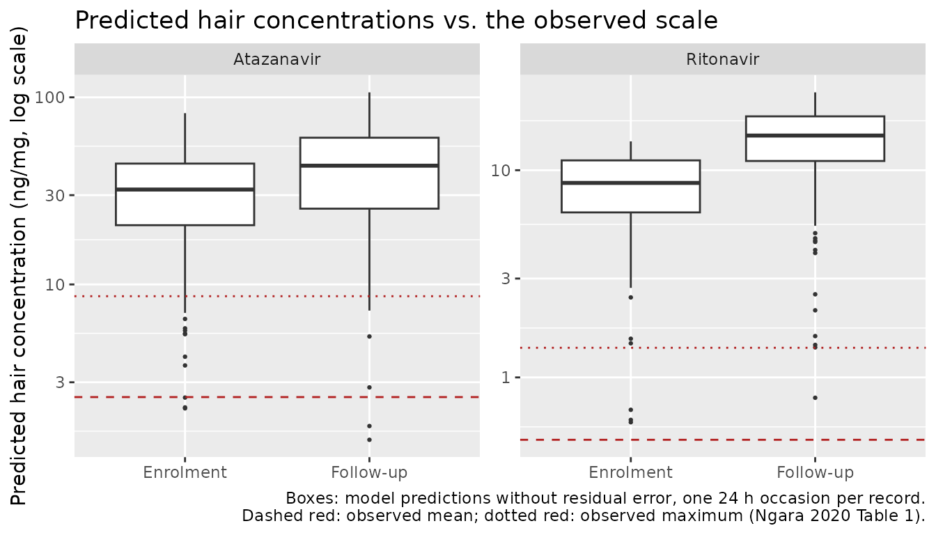
Known deviation: absolute hair level

The packaged models reproduce the paper’s printed parameters, but those parameters do not reproduce the paper’s own observations. With the stated 300 mg atazanavir dose, the typical prediction 24 h after a dose is Frac times the roughly 290 mg eliminated, about 46 ng/mg at the reference covariates. That is roughly 18-fold above the observed mean of 2.5 ng/mg and 5-fold above the highest observed value. For ritonavir 100 mg the typical prediction is about 17 ng/mg against an observed mean of 0.5 ng/mg, roughly 34-fold. At the cohort’s typical covariate values the only downward multipliers are 0.70 or 0.58 (enrolment), 0.79 (overweight) and 0.46 (sibling caregiver), so the reported covariate effects cannot close the gap. The two drugs are also off by different factors, so a single unit slip does not explain it. Treating the 24 h sample as one dosing interval at steady state gives nearly the same value, Frac times the dose (48 and 18 ng/mg). The paper’s dosing-record and unit conventions are not published and no control stream is available, so the models are shipped exactly as printed. The covariate effects, which are the paper’s main results, are relative and unaffected. The check below pins this documented state: it fails if a future change to the models brings the absolute level onto the observed scale, at which point this section must be rewritten.

stopifnot(all(hair_summary$fold_over_observed_mean > 5))

The paper’s prose also describes Frac as hair concentration “approximately 16% the amount of atazanavir plasma trough concentration”. That reading contradicts Equation 3 in the other direction. The typical steady-state atazanavir trough under the fixed plasma parameters is about 0.17 mg/L, and 16% of it is far below both the model prediction and the observed hair concentrations.

Plasma layer: PKNCA at steady state

The fixed plasma parameters are the only part of the models that a classical NCA can check. Over one dosing interval at steady state, AUCtau must equal Dose / (CL/F) for each simulated participant. The models are dosed once daily for 21 days and the last interval (480-504 h) is analysed with PKNCA, grouped by drug.

ss_events <- function(dose) {
  dose_rows <- tibble(time = seq(0, 480, by = 24), evid = 1L, amt = dose,
                      cmt = "depot")
  obs_rows <- tibble(time = seq(480, 504, by = 0.25), evid = 0L, amt = 0,
                     cmt = "central")
  subjects |>
    mutate(id = subject, OCC = 2) |>
    tidyr::crossing(bind_rows(dose_rows, obs_rows)) |>
    arrange(id, time, desc(evid)) |>
    as.data.frame()
}

sim_ss <- bind_rows(
  rxode2::rxSolve(mod_atv, events = ss_events(300), maxsteps = 1e6) |>
    as.data.frame() |>
    mutate(drug = "Atazanavir", dose = 300),
  rxode2::rxSolve(mod_rtv, events = ss_events(100), maxsteps = 1e6) |>
    as.data.frame() |>
    mutate(drug = "Ritonavir", dose = 100)
) |>
  mutate(id = ifelse(drug == "Ritonavir", id + 1000L, id))

stopifnot(all(sim_ss$Cc >= -1e-6 * max(sim_ss$Cc, na.rm = TRUE), na.rm = TRUE))

conc_df <- sim_ss |>
  filter(!is.na(Cc)) |>
  mutate(Cc = pmax(Cc, 0)) |>
  select(id, time, Cc, drug)

dose_df <- bind_rows(
  ss_events(300) |> mutate(drug = "Atazanavir"),
  ss_events(100) |> mutate(drug = "Ritonavir", id = id + 1000L)
) |>
  filter(evid == 1) |>
  select(id, time, amt, drug)

conc_obj <- PKNCA::PKNCAconc(conc_df, Cc ~ time | drug + id)
dose_obj <- PKNCA::PKNCAdose(dose_df, amt ~ time | drug + id)
intervals <- data.frame(start = 480, end = 504, auclast = TRUE, cmax = TRUE,
                        tmax = TRUE, cmin = TRUE)
nca_res <- PKNCA::pk.nca(PKNCA::PKNCAdata(conc_obj, dose_obj, intervals = intervals))

nca_wide <- as.data.frame(nca_res) |>
  select(drug, id, PPTESTCD, PPORRES) |>
  tidyr::pivot_wider(names_from = PPTESTCD, values_from = PPORRES)

auc_check <- nca_wide |>
  left_join(
    sim_ss |> group_by(drug, id) |> summarise(cl = first(cl), dose = first(dose),
                                              .groups = "drop"),
    by = c("drug", "id")
  ) |>
  mutate(auc_expected = dose / cl, pct_diff = 100 * (auclast / auc_expected - 1))

auc_check |>
  group_by(drug) |>
  summarise(
    cmax_median = median(cmax), tmax_median = median(tmax),
    cmin_median = median(cmin), auctau_median = median(auclast),
    dose_over_cl_median = median(auc_expected),
    median_abs_pct_diff = median(abs(pct_diff)),
    .groups = "drop"
  ) |>
  dplyr::rename(
    "Drug" = drug, "Cmax (mg/L)" = cmax_median, "Tmax (h)" = tmax_median,
    "Cmin (mg/L)" = cmin_median, "AUCtau (mg*h/L)" = auctau_median,
    "Dose / CL (mg*h/L)" = dose_over_cl_median,
    "Median |AUCtau vs Dose/CL| (%)" = median_abs_pct_diff
  ) |>
  knitr::kable(digits = 3,
               caption = "Steady-state plasma NCA (day 21), medians over 200 simulated participants per drug.")

Steady-state plasma NCA (day 21), medians over 200 simulated participants per drug.
Drug	Cmax (mg/L)	Tmax (h)	Cmin (mg/L)	AUCtau (mg*h/L)	Dose / CL (mg*h/L)	Median \|AUCtau vs Dose/CL\| (%)
Atazanavir	4.711	3.125	0.202	46.911	46.994	0.058
Ritonavir	0.882	1.250	0.063	8.433	8.496	0.145


# Same drawn parameters on both sides; the residual is trapezoid error on the
# 0.25 h grid plus the last few percent of accumulation for the slowest
# clearances (CL/F IIV variance 1.04 for atazanavir).
stopifnot(
  abs(median(auc_check$pct_diff)) < 1,
  quantile(abs(auc_check$pct_diff), 0.9) < 3
)

The paper reports no plasma NCA, so there is no published comparison table. For the typical 70 kg participant the fixed atazanavir parameters give AUCtau = 300 / 10 = 30 mgh/L, and the fixed ritonavir parameters give 100 / 12.8 = 7.8 mgh/L.

sim_ss |>
  filter(!is.na(Cc)) |>
  group_by(drug, time) |>
  summarise(
    Q05 = quantile(Cc, 0.05), Q50 = median(Cc), Q95 = quantile(Cc, 0.95),
    .groups = "drop"
  ) |>
  ggplot(aes(time - 480, Q50)) +
  geom_ribbon(aes(ymin = Q05, ymax = Q95), alpha = 0.25) +
  geom_line() +
  facet_wrap(~drug, scales = "free_y") +
  labs(x = "Time after the day-21 dose (h)", y = "Plasma Cc (mg/L)",
       title = "Steady-state plasma profiles implied by the fixed parameters",
       caption = "Median and 90% interval, 200 simulated participants per drug.")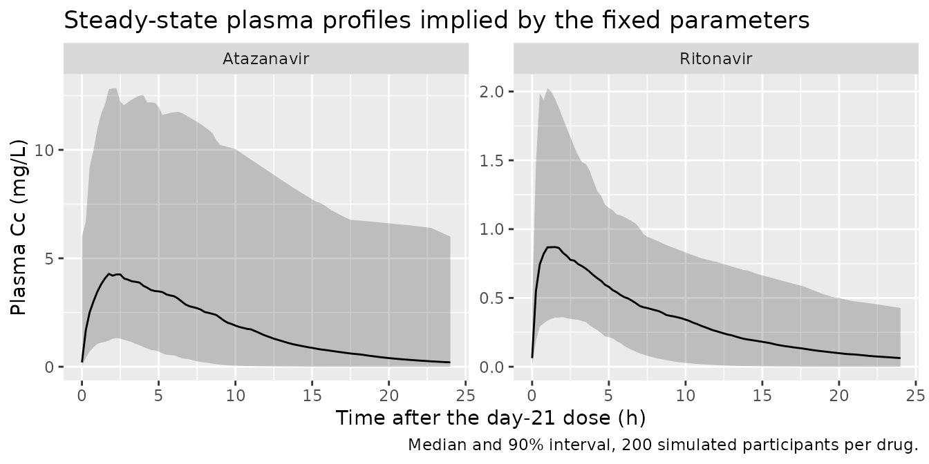

Assumptions and deviations

Absolute hair level does not match the paper’s data. The printed parameters predict hair concentrations about 18-fold (atazanavir) and 34-fold (ritonavir) above the observed means (see “Known deviation” above). The models are encoded exactly as printed and nothing is tuned. Relative covariate effects are unaffected.
Occasion coding. Each hair sample is simulated as one dose at time 0 with a sample 24 h later and an empty hair compartment, as Figure 2’s sampling times suggest. The paper does not say how the enrolment hair content was handled at the follow-up record. Under the model’s no-loss structure, carrying it over would roughly double the follow-up prediction.
Reference weight. Allometric scaling of the atazanavir CL/F and Vc is stated, but the reference weight and the cohort’s weights are not. 70 kg is used. The Discussion mentions adjustment “by the median body weight observed in our study”, which is not printed. Because the hair amount is a fraction of the drug eliminated, the 24 h hair prediction is insensitive to this choice.
No weight scaling for ritonavir. The ritonavir paragraph lists the fixed plasma values without a weight term, so none is applied.
Adherence centring. The PsN linear form 1 + theta * (VAS - centre) needs a centring value that is not printed. The rounded cohort mean, 84, is used. With the printed coefficient of 0.02, the factor falls to zero at a VAS of 34 and is negative below it. The cohort’s minimum VAS is 30, so the model as printed predicts a negative hair-deposition fraction, and a negative hair concentration, for the least adherent participants. The model is not clamped, so users simulating low adherence should note this. The bootstrap results point to a likely explanation. PsN’s stepwise covariate search bounds a linear continuous coefficient so that the factor stays non-negative over the observed range, which caps it at 1 / (median - minimum). Both drugs’ bootstrap 90% intervals end at 0.017, close to 1 / (90 - 30) = 0.0167. That is consistent with a cohort median VAS near 90 and an estimate at the bound, printed rounded as 0.02. Neither the median nor the unrounded estimate is printed, so the published values are kept.
Variability column. The Tables 3 and 5 ‘Variability’ entries are read as NONMEM omega-squared values on log-normal parameters. The Methods mention inter-occasion variability, but the tables report a single variability column, which is encoded as between-subject variability. The atazanavir bootstrap column prints 0.44 for the fixed k12 variability, against 0.45 in the estimate column. The estimate column is used.
k12 units. The tables print k12 in ‘litres hour-1’. As an absorption rate constant, k12 is encoded in 1/h.
Residual error. ‘eps ADD’ and ‘eps PROP’ are read as additive (ng/mg) and proportional standard deviations with sigma fixed to 1, i.e. a combined error model.
Virtual-cohort covariates. Body weight (not reported) is drawn around 45 kg. The other covariates follow Table 1 frequencies. Table 1 counts 46 participants with a BMI-for-age category, and those 46 set the category frequencies.
Errata. No correction notice for this article was found on the journal site or PubMed as of 2026-10-16.