Rilpivirine (Thoueille 2024)
Source:vignettes/articles/Thoueille_2024_rilpivirine.Rmd
Thoueille_2024_rilpivirine.RmdModel and source
#> ℹ parameter labels from comments will be replaced by 'label()'
#> Warning: some etas defaulted to non-mu referenced, possible parsing error: etaiov_cl_1, etaiov_cl_2, etaiov_cl_3, etaiov_cl_4, etaiov_cl_5, etaiov_cl_6
#> as a work-around try putting the mu-referenced expression on a simple line
Citation: Thoueille P, Saldanha SA, Schaller F, Choong E, Veuve F, Munting A, Cavassini M, Braun D, Gunthard HF, Duran Ramirez JJ, Surial B, Furrer H, Rauch A, Ustero P, Calmy A, Stockle M, Di Benedetto C, Bernasconi E, Schmid P, Marzolini C, Girardin FR, Buclin T, Decosterd LA, Guidi M; for the Swiss HIV Cohort Study. Population pharmacokinetics of rilpivirine following oral administration and long-acting intramuscular injection in real-world people with HIV. Front Pharmacol. 2024;15:1437400. doi:10.3389/fphar.2024.1437400.
Description: Two-compartment population PK model for rilpivirine covering both the oral 25 mg daily lead-in and the long-acting intramuscular nanosuspension in people with HIV followed in routine clinical care in the Swiss HIV Cohort Study (Thoueille 2024). Oral doses enter the central compartment as a zero-order input of duration Doral fixed to 4 h and carry a relative bioavailability Foral = 65.4% with between-subject variability; the intramuscular injection is assumed completely bioavailable and is split between two parallel first-order release pathways, a fast pathway taking a fraction Fi.m.fast = 27.6% of the dose with kafast = 0.00214 1/h and a slow pathway taking the remainder with kaslow = 0.000229 1/h. Because both absorption rate constants are far below the elimination rate constant, long-acting rilpivirine shows flip-flop kinetics with an apparent half-life of 18 weeks driven by kaslow. Clearance carries both between-subject and inter-occasion variability across up to six injection occasions, and the residual error switches by route: additive after oral dosing and proportional after intramuscular injection. No covariate was retained in the final validated model; a female-sex effect reducing Fi.m.fast by 45.6% was estimated but judged not clinically relevant and left out (see covariatesDataExcluded).
Supplement (open access, contains the final NONMEM control stream): https://www.frontiersin.org/articles/10.3389/fphar.2024.1437400/full#supplementary-material
Rilpivirine is a non-nucleoside reverse-transcriptase inhibitor given either as a 25 mg daily oral tablet or, combined with cabotegravir, as a long-acting intramuscular nanosuspension. Thoueille 2024 is the first population PK analysis of long-acting rilpivirine in a routine-care cohort rather than in the phase III registrational trials, and it is unusual in fitting the oral and the intramuscular routes jointly in a single model.
Population
The analysis pooled 238 people with HIV enrolled in a nationwide Swiss observational study nested in the Swiss HIV Cohort Study, contributing 1038 rilpivirine plasma concentrations: 186 after oral administration (from 176 people) and 852 after intramuscular injection (from 222 people), with detailed within-interval sampling in 28 people (Thoueille 2024 Results, first paragraph). The median number of samples per person was 4 (range 1 to 15) and the median follow-up was 26 weeks (range 3 to 196). Only 10 people had concentrations that could be assumed to be at intramuscular steady state, i.e. from week 96.
Baseline characteristics come from Thoueille 2024 Table 1: 190 men (80%) and 48 women (20%); median age 46 years (20 to 79); median body weight 78 kg (50 to 126); median height 176 cm (151 to 198); median BMI 25.4 kg/m^2 (18.2 to 43.3). Ethnicity was White in 133 (56%), Black in 36 (15%), Hispanic American in 19 (8%), Asian in 11 (5%) and other or missing in 39 (16%). CKD-EPI eGFR was category G1 in 158 (66%), G2 in 76 (32%) and G3 in 4 (2%). Plasma HIV RNA was below 50 copies/mL in 233 (98%) and CD4 count was at least 500 cells/mm^3 in 186 (78%). Two people had Child-Pugh class A cirrhosis.
The same information is available programmatically via the model’s
population metadata
(rxode2::rxode(readModelDb("Thoueille_2024_rilpivirine"))$population).
#> List of 18
#>  $ species       : chr "human"
#>  $ n_subjects    : int 238
#>  $ n_studies     : int 1
#>  $ n_observations: chr "1038 rilpivirine plasma concentrations: 186 after oral administration from 176 people and 852 after intramuscul"| __truncated__
#>  $ age_range     : chr "20-79 years (median 46; Thoueille 2024 Table 1)"
#>  $ age_median    : chr "46 years"
#>  $ weight_range  : chr "50-126 kg (median 78; Thoueille 2024 Table 1)"
#>  $ weight_median : chr "78 kg"
#>  $ height_range  : chr "151-198 cm (median 176; Thoueille 2024 Table 1)"
#>  $ bmi_range     : chr "18.2-43.3 kg/m^2 (median 25.4; Thoueille 2024 Table 1). BMI < 25 in 104 (44%), 25-30 in 103 (43%), > 30 in 31 ("| __truncated__
#>  $ sex_female_pct: num 20.2
#>  $ race_ethnicity: Named num [1:5] 56 15 8 5 16
#>  $ disease_state : chr "People with HIV-1 on suppressive antiretroviral therapy switching to, or established on, long-acting cabotegrav"| __truncated__
#>  $ renal_function: chr "CKD-EPI eGFR category G1 (>= 90 mL/min/1.73m^2) in 158 (66%), G2 (60-89) in 76 (32%), G3 (30-59) in 4 (2%)"
#>  $ dose_range    : chr "Oral rilpivirine 25 mg once daily during the lead-in; long-acting intramuscular gluteal rilpivirine 900 mg with"| __truncated__
#>  $ regions       : chr "Switzerland (Lausanne, Zurich, Bern, Geneva, Basel, Lugano, St Gallen)"
#>  $ co_medication : chr "Cabotegravir is co-administered in every intramuscular injection. Thoueille 2024 Methods state that no clinical"| __truncated__
#>  $ notes         : chr "Real-world therapeutic-drug-monitoring cohort nested in the Swiss HIV Cohort Study, sampled mostly sparsely at "| __truncated__
Structural model
Thoueille 2024 Figure 1 and the supplementary control stream describe a four-compartment system:
- An oral dose enters the central
compartment as a zero-order input of duration
Doral, fixed at 4 h, scaled by a relative bioavailabilityForal= 65.4%. Intramuscular administration is taken as completely bioavailable, soForalis the oral-to-intramuscular ratio. - An intramuscular dose is split between two parallel
first-order release pathways: a fraction
Fi.m.fast= 27.6% throughdepotwithkafast= 0.00214 1/h, and the remainder throughdepot2withkaslow= 0.000229 1/h. The fast fraction is carried on the logit scale so it cannot leave (0, 1). - Disposition is two-compartment:
central(V3 = 277 L) exchanges withperipheral1(V4 = 839 L) through Q = 4.08 L/h and is cleared at CL = 6.74 L/h.
Because both absorption rate constants are far smaller than the
elimination rate constant, long-acting rilpivirine displays flip-flop
kinetics: the apparent terminal half-life is set by kaslow,
not by CL/V.
Two model-level details are worth stating explicitly.
-
The route indicator is only read by the error
model. In the source control stream,
LAIdoes two jobs: it selects the absorption block in$PKand the residual-error branch in$ERROR. Here the absorption branch is carried by the dose record’s target compartment instead (an oral record goes intocentralwithrate = -2; an intramuscular record goes intodepotanddepot2), so the packaged model readsROUTE_ORALonly to choose between the additive oral SD and the proportional intramuscular SD.ROUTE_ORAL = 1 - LAI. -
Inter-occasion variability on CL uses six occasion
slots. The control stream’s
$ABBR REPLACE ETA(OCC)=ETA(5,6,7,8,9,10), backed by one$OMEGA BLOCK(1) 0.0167and fiveSAMElines, means all six occasions share a single variance. Occasions 2 to 6 are thereforefixed()at the estimated occasion-1 variance.
Source trace
Every ini() entry in
inst/modeldb/specificDrugs/Thoueille_2024_rilpivirine.R
carries an in-file comment naming its origin. They are collected here
for review. “Table 2” is Thoueille 2024 Table 2 (“Final population PK
parameter estimates of rilpivirine with their bootstrap evaluations”);
“control stream” is the NONMEM CODE FOR FINAL MODEL listing
on pages 7 to 9 of the open-access Supplementary Information.
| Equation / parameter | Value | Source location |
|---|---|---|
lcl (CL) |
6.74 L/h | Table 2 row CL (L/h), RSE 5%; control stream
$THETA(1)
|
lvc (V3) |
277 L | Table 2 row V 3 (L), RSE 25%; control stream
$THETA(2)
|
lq (Q) |
4.08 L/h | Table 2 row Q (L/h), RSE 40%; control stream
$THETA(3)
|
lvp (V4) |
839 L | Table 2 row V 4 (L), RSE 11%; control stream
$THETA(4)
|
lfdepot_oral (Foral) |
0.654 | Table 2 row F oral (%) = 65.4, RSE 5%; control stream
$THETA(5)
|
logitfdepot (Fi.m.fast) |
logit(0.276) | Table 2 row F i.m.fast (%) = 27.6, RSE 9%; control
stream $THETA(6)
|
ld1_oral (Doral) |
4 h, fixed | Table 2 row D oral (h) 4 FIX; control stream
$THETA(7) 4 FIX; Methods paragraph 2 of “Model building and
selection” |
lka (kafast) |
0.00214 1/h | Table 2 row k a fast (h-1), RSE 11%; control stream
$THETA(8)
|
lka2 (kaslow) |
0.000229 1/h | Table 2 row k a slow (h-1), RSE 11%; control stream
$THETA(9)
|
etalcl |
0.0649 | control stream $OMEGA IIV CL; equals Table
2 omega CL (CV%) 25.9
|
etalfdepot_oral |
0.129 | control stream $OMEGA IIV F3; equals Table
2 omega F oral (CV%) 37.1
|
etalogitfdepot |
0.708 | control stream $OMEGA IIV F1; equals Table
2 omega F i.m.fast (CV%) 16.8 under the Table 2 footnote-c
approximation |
etalka2 |
0.521 | control stream $OMEGA IIV KA2 LAI; equals
Table 2 omega k a slow (CV%) 82.7
|
etaiov_cl_1 .. etaiov_cl_6
|
0.0167 | control stream $OMEGA BLOCK(1) 0.0167 + five
SAME; equals Table 2 omega IOV (CV%) 13.0
|
addSdOral |
sqrt(317) = 17.80 ng/mL | control stream $SIGMA 317 ; Add PO; Table 2
sigma add-oral (ng/mL) 18
|
propSdIm |
sqrt(0.031) = 0.1761 | control stream $SIGMA 0.031 ; Prop LAI; Table 2
sigma prop-LA (CV%) 18
|
| ODE system | n/a | control stream $DES, DADT(1) to
DADT(4); Thoueille 2024 Figure 1 |
Logit parameterisation of Fi.m.fast
|
n/a | Thoueille 2024 Methods, “Model building and selection”, displayed
equation for TEMP; control stream $PK
TEMP = LOG(THETA(6)/(1-THETA(6)))
|
| ng/mL scaling | Cc = 1000 * central / vc |
control stream $PK S3 = V3/1000
|
Sex effect on Fi.m.fast (NOT in the model) |
-45.6% | Thoueille 2024 Results 3.1; commented out in the control stream. See “Assumptions and deviations” |
The between-subject variance scale is the one place where Table 2 and the control stream report different quantities, so it is checked explicitly rather than assumed.
# Table 2 prints CV%; the control stream prints the underlying $OMEGA variance.
# Each row below re-derives the printed CV% from the variance actually encoded
# in ini(), under the transformation that row's parameter uses. A mis-scaled
# omega (variance entered as an SD, or a CV entered as a variance) fails here.
ini_df <- ui$iniDf
om <- function(nm) ini_df$est[!is.na(ini_df$name) & ini_df$name == nm]

logn_cv <- function(v) sqrt(exp(v) - 1) * 100
# Table 2 footnote c: CV(Fi.m.fast) is approximated as theta * (1 - theta) * omega
theta_fast <- 0.276
logit_cv <- function(v) theta_fast * (1 - theta_fast) * sqrt(v) * 100

omega_check <- tibble::tibble(
  Parameter = c("CL", "Foral", "Fi.m.fast", "kaslow", "IOV on CL"),
  `Encoded variance` = c(om("etalcl"), om("etalfdepot_oral"),
                         om("etalogitfdepot"), om("etalka2"), om("etaiov_cl_1")),
  `Derived CV%` = c(logn_cv(om("etalcl")), logn_cv(om("etalfdepot_oral")),
                    logit_cv(om("etalogitfdepot")), logn_cv(om("etalka2")),
                    logn_cv(om("etaiov_cl_1"))),
  `Table 2 CV%` = c(25.9, 37.1, 16.8, 82.7, 13.0)
)
omega_check$`Abs diff` <- abs(omega_check$`Derived CV%` - omega_check$`Table 2 CV%`)

# Deterministic: these come from ini() and Table 2, not from a simulation, so a
# tight bound is correct. Table 2 rounds to one decimal, so 0.05 is the rounding
# half-width; 0.1 leaves room for that without admitting a real mis-scaling
# (entering an SD as a variance moves these by tens of CV points).
stopifnot(max(omega_check$`Abs diff`) < 0.1)

knitr::kable(omega_check, digits = 4,
caption = "Between-subject and inter-occasion variance scale checked against Thoueille 2024 Table 2.")| Parameter | Encoded variance | Derived CV% | Table 2 CV% | Abs diff |
|---|---|---|---|---|
| CL | 0.0649 | 25.8945 | 25.9 | 0.0055 |
| Foral | 0.1290 | 37.1066 | 37.1 | 0.0066 |
| Fi.m.fast | 0.7080 | 16.8137 | 16.8 | 0.0137 |
| kaslow | 0.5210 | 82.6868 | 82.7 | 0.0132 |
| IOV on CL | 0.0167 | 12.9770 | 13.0 | 0.0230 |
Closed-form checks against the paper’s own derived quantities
Thoueille 2024 Discussion reports several quantities derived from the
parameter estimates rather than estimated directly. They are reproduced
here from the packaged ini() values, which makes each one a
live check on the transcription: a mis-typed clearance or volume moves
the disposition half-lives by tens of percent.
th <- function(nm) ini_df$est[!is.na(ini_df$name) & ini_df$name == nm]
cl <- exp(th("lcl")); vc <- exp(th("lvc"))
q  <- exp(th("lq"));  vp <- exp(th("lvp"))
ka_fast <- exp(th("lka")); ka_slow <- exp(th("lka2"))

kel <- cl / vc; k12 <- q / vc; k21 <- q / vp
sum_k <- kel + k12 + k21
disc  <- sqrt(sum_k^2 - 4 * kel * k21)
alpha <- (sum_k + disc) / 2
beta  <- (sum_k - disc) / 2

WK <- 168  # h per week

derived <- tibble::tibble(
  Quantity = c("Oral distribution half-life (h)",
               "Oral terminal disposition half-life (h)",
               "Long-acting apparent half-life, log(2)/kaslow (weeks)",
               "Time to steady state, 5 x log(2)/kaslow (years)",
               "kafast / kel (unitless)",
               "kaslow / kel (unitless)"),
  Model = c(log(2) / alpha, log(2) / beta, log(2) / ka_slow / WK,
            5 * log(2) / ka_slow / (WK * 52), ka_fast / kel, ka_slow / kel),
  Paper = c(17, 240, 18.0, 1.7, NA, NA),
  Source = c("Discussion paragraph 4", "Discussion paragraph 4",
             "Discussion paragraph 4 (90% CI 5.5 to 59.0)",
             "Discussion paragraph 4 (90% CI 0.5 to 5.7)",
             "Results 3.1 'flip-flop' kinetics", "Results 3.1 'flip-flop' kinetics")
)

# Deterministic arithmetic on ini() values versus numbers PRINTED in the paper,
# so these can go red if a parameter is mis-transcribed. Tolerances are the
# printed rounding widths, not a fitted-to-this-run bound.
stopifnot(
  abs(derived$Model[1] - 17)   < 0.5,   # printed to 2 significant figures
  abs(derived$Model[2] - 240)  < 5,     # printed to 3 significant figures
  abs(derived$Model[3] - 18.0) < 0.2,   # printed to 3 significant figures
  abs(derived$Model[4] - 1.7)  < 0.1,
  # Flip-flop: Results 3.1 states both absorption rate constants are BELOW the
  # elimination rate constant. Both are in fact roughly one and two orders of
  # magnitude below it.
  derived$Model[5] < 0.2,
  derived$Model[6] < 0.02
)

knitr::kable(derived, digits = c(NA, 3, 1, NA),
caption = "Derived quantities reproduced from the packaged ini() values.")| Quantity | Model | Paper | Source |
|---|---|---|---|
| Oral distribution half-life (h) | 16.889 | 17.0 | Discussion paragraph 4 |
| Oral terminal disposition half-life (h) | 240.418 | 240.0 | Discussion paragraph 4 |
| Long-acting apparent half-life, log(2)/kaslow (weeks) | 18.017 | 18.0 | Discussion paragraph 4 (90% CI 5.5 to 59.0) |
| Time to steady state, 5 x log(2)/kaslow (years) | 1.732 | 1.7 | Discussion paragraph 4 (90% CI 0.5 to 5.7) |
| kafast / kel (unitless) | 0.088 | NA | Results 3.1 ‘flip-flop’ kinetics |
| kaslow / kel (unitless) | 0.009 | NA | Results 3.1 ‘flip-flop’ kinetics |
Virtual cohort
Original observed data are not publicly available. The final model
carries no demographic covariates, so the only structure a virtual
cohort needs is the dosing regimen and the row-level
ROUTE_ORAL and OCC columns.
Two arms are simulated, 200 participants each (the per-arm cap for these vignettes; the extra precision of a larger cohort adds nothing to the checks below):
- Long-acting arm – the regimen Thoueille 2024 Figure 2 and Supplementary Table S2 simulate: a 4-week oral lead-in of 25 mg once daily, then 900 mg intramuscular at week 4, again at week 8, and every 8 weeks thereafter. The published trough time points (weeks 8, 16, 24, 32, 40 and 48) then fall exactly at the end of each dosing interval, and week 8 is “4 weeks after the loading dose” as the paper describes it.
- Oral arm – 25 mg once daily for 24 weeks, reproducing the oral steady-state profile of Supplementary Figure S2. Twenty-four weeks is about 17 terminal disposition half-lives, so the last interval is genuinely at steady state.
# set.seed() seeds R's RNG, NOT rxode2's simulation RNG, and rxode2's streams
# are partitioned per solver thread. The cohort below therefore differs between
# a 16-thread workstation and a 2-core CI runner and no seed can make them
# agree. Every assertion downstream is written to hold for any cohort this
# model can produce.
set.seed(20260906)
rxode2::rxSetSeed(20260906)

n_per_arm <- 200L

# --- Long-acting arm ---------------------------------------------------------
inj_times <- c(4, 8, 16, 24, 32, 40, 48) * WK
lai_ev <- rxode2::et(amt = 25, cmt = "central", rate = -2,
                     time = 0, ii = 24, addl = 27)
for (tt in inj_times) {
  # One injection is entered as TWO simultaneous records carrying the full
  # 900 mg; f(depot) and f(depot2) in the model split it into the fast and
  # slow release pathways.
  lai_ev <- rxode2::et(lai_ev, amt = 900, cmt = "depot",  time = tt)
  lai_ev <- rxode2::et(lai_ev, amt = 900, cmt = "depot2", time = tt)
}
lai_obs <- sort(unique(c(seq(0, 52 * WK, by = 24), inj_times,
                         c(8, 16, 24, 32, 40, 48) * WK)))
lai_ev <- rxode2::et(lai_ev, lai_obs)

lai_events <- as.data.frame(lai_ev) |>
  dplyr::mutate(
    arm        = "Long-acting IM 900 mg",
    ROUTE_ORAL = as.numeric(time < 4 * WK),
    # Occasion 1 covers the oral lead-in and the first injection interval;
    # each later injection starts a new occasion, capped at the six slots the
    # source model allocates.
    OCC        = pmin(pmax(findInterval(time, inj_times[1:6]), 1L), 6L)
  )

# --- Oral arm ----------------------------------------------------------------
oral_last_dose <- 167 * 24                      # last of 168 daily doses
oral_ev <- rxode2::et(amt = 25, cmt = "central", rate = -2,
                      time = 0, ii = 24, addl = 167)
oral_obs <- sort(unique(c(seq(0, oral_last_dose, by = 24),
                          oral_last_dose + seq(0, 24, by = 0.25))))
oral_ev <- rxode2::et(oral_ev, oral_obs)

oral_events <- as.data.frame(oral_ev) |>
  dplyr::mutate(arm = "Oral 25 mg QD", ROUTE_ORAL = 1, OCC = 1L)

stopifnot(
  all(c("ROUTE_ORAL", "OCC") %in% names(lai_events)),
  all(lai_events$OCC >= 1L & lai_events$OCC <= 6L),
  # Every observation row must target an ODE state, never the observable `Cc`.
  all(is.na(lai_events$cmt) |
        lai_events$cmt %in% c("depot", "depot2", "central", "peripheral1"))
)
Simulation
The two arms are solved separately because they have different event
tables, then given disjoint subject-ID ranges so they can be pooled for
the NCA without rxSolve merging subjects.
mod <- readModelDb("Thoueille_2024_rilpivirine")

sim_lai <- rxode2::rxSolve(mod, lai_events, nSub = n_per_arm,
                           addDosing = FALSE) |>
  as.data.frame() |>
  dplyr::mutate(id = as.integer(sim.id), arm = "Long-acting IM 900 mg")
#> ℹ parameter labels from comments will be replaced by 'label()'
#> Warning: some etas defaulted to non-mu referenced, possible parsing error: etaiov_cl_1, etaiov_cl_2, etaiov_cl_3, etaiov_cl_4, etaiov_cl_5, etaiov_cl_6
#> as a work-around try putting the mu-referenced expression on a simple line

sim_oral <- rxode2::rxSolve(mod, oral_events, nSub = n_per_arm,
                            addDosing = FALSE) |>
  as.data.frame() |>
  dplyr::mutate(id = as.integer(sim.id) + n_per_arm, arm = "Oral 25 mg QD")

stopifnot(
  length(intersect(sim_lai$id, sim_oral$id)) == 0L,
  all(is.finite(sim_lai$Cc)), all(sim_lai$Cc >= 0),
  all(is.finite(sim_oral$Cc)), all(sim_oral$Cc >= 0)
)
Replicate published figures
Figure 2 – long-acting profile after a 4-week oral lead-in
# Replicates Figure 2 of Thoueille 2024: simulated population percentiles after
# intramuscular administration following a 4-week oral lead-in, with the
# PAIC90 (12 ng/mL, dashed) and the therapeutic-response threshold
# (50 ng/mL, dotted).
pct_lai <- sim_lai |>
  dplyr::group_by(time) |>
  dplyr::summarise(
    Q025 = quantile(Cc, 0.025), Q25 = quantile(Cc, 0.25),
    Q50  = quantile(Cc, 0.50),
    Q75  = quantile(Cc, 0.75),  Q975 = quantile(Cc, 0.975),
    .groups = "drop"
  ) |>
  dplyr::mutate(week = time / WK)

ggplot(pct_lai, aes(week, Q50)) +
  geom_ribbon(aes(ymin = Q025, ymax = Q975), fill = "grey80") +
  geom_ribbon(aes(ymin = Q25, ymax = Q75), fill = "grey55") +
  geom_line(colour = "white", linewidth = 0.8) +
  geom_hline(yintercept = 12, linetype = "dashed") +
  geom_hline(yintercept = 50, linetype = "dotted") +
  scale_y_log10() +
  labs(x = "Time since treatment initiation (weeks)",
       y = "Rilpivirine concentration (ng/mL)",
       title = "Figure 2 -- long-acting rilpivirine population percentiles",
       caption = paste("Replicates Figure 2 of Thoueille 2024.",
                       "Dashed line PAIC90 = 12 ng/mL; dotted line 50 ng/mL."))
#> Warning in scale_y_log10(): log-10 transformation introduced infinite values.
#> log-10 transformation introduced infinite values.
#> log-10 transformation introduced infinite values.
#> log-10 transformation introduced infinite values.
#> log-10 transformation introduced infinite values.
#> log-10 transformation introduced infinite values.
#> log-10 transformation introduced infinite values.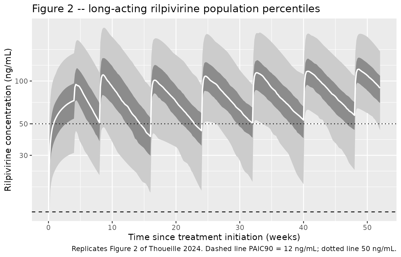
Figure S2 – oral profile at steady state
# Replicates Supplementary Figure S2 of Thoueille 2024 over the final 24 h
# dosing interval of the oral arm.
sim_oral |>
  dplyr::filter(time >= oral_last_dose) |>
  dplyr::mutate(tad = time - oral_last_dose) |>
  dplyr::group_by(tad) |>
  dplyr::summarise(
    Q025 = quantile(Cc, 0.025), Q25 = quantile(Cc, 0.25),
    Q50  = quantile(Cc, 0.50),
    Q75  = quantile(Cc, 0.75),  Q975 = quantile(Cc, 0.975),
    .groups = "drop"
  ) |>
  ggplot(aes(tad, Q50)) +
  geom_ribbon(aes(ymin = Q025, ymax = Q975), fill = "grey80") +
  geom_ribbon(aes(ymin = Q25, ymax = Q75), fill = "grey55") +
  geom_line(colour = "white", linewidth = 0.8) +
  geom_hline(yintercept = 12, linetype = "dashed") +
  geom_hline(yintercept = 50, linetype = "dotted") +
  labs(x = "Time after dose (h)", y = "Rilpivirine concentration (ng/mL)",
       title = "Figure S2 -- oral rilpivirine 25 mg once daily at steady state",
       caption = "Replicates Supplementary Figure S2 of Thoueille 2024.")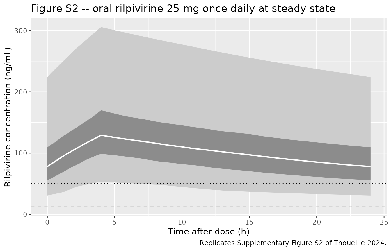
PKNCA validation
NCA is run over one dosing interval per published trough time point,
plus the final oral dosing interval, so that PKNCA’s
ctrough – the end-of-interval concentration – is exactly
the quantity Thoueille 2024 Supplementary Table S2 tabulates.
cmin is requested alongside it but is a different quantity
here: over the week 4 to week 8 interval the profile still carries the
tail of the oral lead-in, so its minimum falls in the middle of the
interval rather than at its end.
windows <- tibble::tribble(
  ~window,       ~arm,                    ~start,   ~end,
  "Week 4-8",    "Long-acting IM 900 mg",  4 * WK,  8 * WK,
  "Week 8-16",   "Long-acting IM 900 mg",  8 * WK, 16 * WK,
  "Week 16-24",  "Long-acting IM 900 mg", 16 * WK, 24 * WK,
  "Week 24-32",  "Long-acting IM 900 mg", 24 * WK, 32 * WK,
  "Week 32-40",  "Long-acting IM 900 mg", 32 * WK, 40 * WK,
  "Week 40-48",  "Long-acting IM 900 mg", 40 * WK, 48 * WK,
  "Oral steady state", "Oral 25 mg QD", oral_last_dose, oral_last_dose + 24
)

sim_all <- dplyr::bind_rows(
  sim_lai  |> dplyr::select(id, time, Cc, arm),
  sim_oral |> dplyr::select(id, time, Cc, arm)
)

# Assign each concentration record to the window it falls in (a record on a
# window boundary belongs to the window that STARTS there, except for the last
# window's closing point which is also that window's trough).
assign_window <- function(df) {
  out <- lapply(seq_len(nrow(windows)), function(i) {
    w <- windows[i, ]
    df |>
      dplyr::filter(arm == w$arm, time >= w$start, time <= w$end) |>
      dplyr::mutate(window = w$window, tad = time - w$start)
  })
  dplyr::bind_rows(out)
}

# Only !is.na(Cc) -- adding `time > 0` or `Cc > 0` would drop the interval-start
# record PKNCA needs to anchor the AUC.
#
# Time is re-based to time-after-dose within each window (`tad`), so every
# window opens at 0 with its dose. This is required, not cosmetic:
# PKNCA::pk.calc.ctrough() finds the trough by `time %in% end`, and PKNCA
# hands it the dose-relative time vector, so an interval expressed in absolute
# study time never matches and every ctrough comes back NA.
sim_nca <- sim_all |>
  dplyr::filter(!is.na(Cc)) |>
  assign_window() |>
  dplyr::arrange(window, id, tad)

stopifnot(nrow(sim_nca) > 0L,
          setequal(unique(sim_nca$window), windows$window),
          all(sim_nca$tad >= 0))

conc_obj <- PKNCA::PKNCAconc(sim_nca, Cc ~ tad | window + id)

# One dose row per subject per window: the injection (or oral tablet) that
# opens that interval, at tad = 0. The event table carries the 900 mg injection
# as two records (depot + depot2); the administered amount is 900 mg, not
# 1800 mg.
dose_df <- windows |>
  dplyr::mutate(amt = ifelse(arm == "Oral 25 mg QD", 25, 900), tad = 0) |>
  dplyr::select(window, tad, amt) |>
  tidyr::crossing(id = sort(unique(sim_nca$id))) |>
  dplyr::inner_join(dplyr::distinct(sim_nca, window, id), by = c("window", "id"))

dose_obj <- PKNCA::PKNCAdose(dose_df, amt ~ tad | window + id)

# `end` must be computed BEFORE `start` is overwritten: dplyr evaluates
# transmute() arguments in order.
intervals <- windows |>
  dplyr::transmute(
    window, end = end - start, start = 0,
    cmax = TRUE, tmax = TRUE, ctrough = TRUE, cmin = TRUE, cav = TRUE,
    auclast = TRUE
  ) |>
  dplyr::select(window, start, end, cmax, tmax, ctrough, cmin, cav, auclast) |>
  as.data.frame()

nca_res <- PKNCA::pk.nca(PKNCA::PKNCAdata(conc_obj, dose_obj,
                                          intervals = intervals))
nca_df <- as.data.frame(nca_res$result)
stopifnot(nrow(nca_df) > 0L)
ctr <- nca_df$PPORRES[nca_df$PPTESTCD == "ctrough"]
# Guard against the silent all-NA ctrough described above: a gate that cannot
# see a value is worse than no gate.
stopifnot(length(ctr) == nrow(windows) * n_per_arm, !anyNA(ctr))
Independent check: average concentration against the closed form
At steady state the average concentration over a dosing interval must
equal Dose * F / (CL * tau) exactly. This compares PKNCA’s
trapezoidal cav against that identity using each
subject’s own drawn CL and Foral, so the only difference is
trapezoidal error on the same curve and a tight bound is the correct
one.
subj_par <- sim_oral |>
  dplyr::distinct(id, cl, fdepot_oral)

cav_cmp <- nca_df |>
  dplyr::filter(window == "Oral steady state", PPTESTCD == "cav") |>
  dplyr::select(id, cav = PPORRES) |>
  dplyr::mutate(id = as.integer(as.character(id))) |>
  dplyr::inner_join(subj_par, by = "id") |>
  dplyr::mutate(
    cav_closed = 1000 * 25 * fdepot_oral / (cl * 24),   # ng/mL
    pct_diff   = 100 * (cav - cav_closed) / cav_closed
  )

stopifnot(nrow(cav_cmp) == n_per_arm)
# Both sides use the SAME drawn parameters, so the residual is pure numerical
# (trapezoidal) error plus the small remaining approach to steady state after
# 24 weeks -- not cohort noise -- and the bound is therefore tight. Measured at
# 1 / 2 / 4 / 16 solver threads: median -0.00056 to -0.00051%, 90th percentile
# of |% difference| 0.0030 to 0.0035%. The bounds below leave more than an
# order of magnitude of headroom over that and still go red on any real error:
# a wrong bioavailability, dose or ng/mL scaling moves cav by tens of percent.
stopifnot(
  abs(median(cav_cmp$pct_diff)) < 0.05,
  quantile(abs(cav_cmp$pct_diff), 0.9) < 0.05
)

tibble::tibble(
  Statistic = c("Median % difference", "90th percentile of |% difference|"),
  Value = c(median(cav_cmp$pct_diff),
            unname(quantile(abs(cav_cmp$pct_diff), 0.9)))
) |>
  knitr::kable(digits = 3,
caption = "PKNCA cav versus Dose * F / (CL * tau) per subject, oral steady state.")| Statistic | Value |
|---|---|
| Median % difference | -0.001 |
| 90th percentile of |% difference| | 0.003 |
Comparison against published trough concentrations
# Thoueille 2024 Supplementary Table S2, row "Model without sex as a covariate"
# -- the row that corresponds to the final validated (covariate-free) model
# encoded here. The Males and Females rows come from the sex-covariate model
# that the authors explicitly did not validate, so they are not the reference.
#
# The oral steady-state trough comes from Thoueille 2024 Results 3.2: "The
# median Ctrough at a steady state under oral rilpivirine was 80 ng/mL
# [95% prediction interval: 32-211]".
published <- tibble::tribble(
  ~window,             ~ctrough,
  "Week 4-8",           50,
  "Week 8-16",          39,
  "Week 16-24",         45,
  "Week 24-32",         50,
  "Week 32-40",         53,
  "Week 40-48",         55,
  "Oral steady state",  80
)

cmp <- nlmixr2lib::ncaComparisonTable(
  simulated = nca_df,
  reference = published,
  by        = "window",
  params    = "ctrough",
  units     = c(ctrough = "ng/mL"),
  tolerance_pct = 20
)

knitr::kable(
  cmp,
  caption = paste("Simulated versus published rilpivirine trough",
                  "concentrations (Thoueille 2024 Supplementary Table S2,",
                  "covariate-free row, and Results 3.2 for the oral value).",
                  "* differs from reference by more than 20%."),
  align = c("l", "l", "r", "r", "r")
)| NCA parameter | window | Reference | Simulated | % diff |
|---|---|---|---|---|
| Ctrough (ng/mL) | Week 4-8 | 50 | 50.8 | +1.6% |
| Ctrough (ng/mL) | Week 8-16 | 39 | 37.4 | -4.1% |
| Ctrough (ng/mL) | Week 16-24 | 45 | 44.4 | -1.3% |
| Ctrough (ng/mL) | Week 24-32 | 50 | 48.9 | -2.1% |
| Ctrough (ng/mL) | Week 32-40 | 53 | 52.7 | -0.5% |
| Ctrough (ng/mL) | Week 40-48 | 55 | 55.2 | +0.4% |
| Ctrough (ng/mL) | Oral steady state | 80 | 79.1 | -1.1% |
# Quantitative gate on the comparison above.
#
# These are medians over a 200-participant cohort drawn from a model whose
# between-subject CV on the trough is large, and the same 200 participants
# supply every window, so the six long-acting rows move together. rxode2's RNG
# streams are partitioned per solver thread, so a CI runner draws a different
# cohort than a workstation does. Measured across 1 / 2 / 4 / 16 threads: the
# median of |% difference| ran 1.18 to 3.07 and the maximum 4.11 to 5.27; four
# different seeds at 16 threads gave per-window differences spanning -7.1% to
# +4.0%. The bounds below sit outside both ranges. Do not tighten them back to
# whatever a single render happens to produce. They still go red on a
# structural error: a mis-transcribed clearance, dose, absorption fraction or
# unit moves the whole trough distribution by tens of percent.
gate <- nca_df |>
  dplyr::filter(PPTESTCD == "ctrough") |>
  dplyr::group_by(window) |>
  dplyr::summarise(sim = median(PPORRES), .groups = "drop") |>
  dplyr::inner_join(published, by = "window") |>
  dplyr::mutate(pct_diff = 100 * (sim - ctrough) / ctrough)

stopifnot(nrow(gate) == nrow(published))
stopifnot(
  median(abs(gate$pct_diff)) < 10,
  max(abs(gate$pct_diff)) < 20
)
Headline simulation claims from the paper
Thoueille 2024 states several proportions in the Results and Abstract. They are checked here as magnitudes with tolerances wide enough to absorb cohort draw, as any assertion on a simulated proportion must be.
trough_at <- function(week) {
  sim_lai$Cc[abs(sim_lai$time - week * WK) < 1e-6]
}
t8  <- trough_at(8)
t16 <- trough_at(16)
stopifnot(length(t8) == n_per_arm, length(t16) == n_per_arm)

claims <- tibble::tibble(
  Claim = c(
    "About 50% of long-acting Ctrough at week 8 exceed 50 ng/mL",
    "Median Ctrough falls about 22% from week 8 to week 16",
    "About 5% of long-acting Ctrough fall below 2 x PAIC90 (24 ng/mL)",
    "About 15% of long-acting Ctrough fall below 32 ng/mL",
    "About 85% of oral Ctrough at steady state exceed 50 ng/mL"
  ),
  Source = c("Results 3.2 / Conclusion", "Results 3.2", "Results 3.2",
             "Results 3.2 / Abstract", "Results 3.2"),
  Paper = c(50, 22, 5, 15, 85),
  Model = c(
    100 * mean(t8 > 50),
    100 * (1 - median(t16) / median(t8)),
    100 * mean(t8 < 24),
    100 * mean(t8 < 32),
    100 * mean(nca_df$PPORRES[nca_df$window == "Oral steady state" &
                                nca_df$PPTESTCD == "ctrough"] > 50)
  )
)

# Percentages of a 200-participant cohort: the binomial standard error alone is
# up to 3.5 points, and the underlying quantiles are steep here, so each bound
# is an absolute-percentage-point window rather than a relative one. Measured
# across 1 / 2 / 4 / 16 solver threads the five model values ran 48.5-52.0,
# 19.6-26.4, 3.0-8.5, 13.5-18.5 and 79.5-81.5, i.e. at most 4.4 points from the
# published value on any row. Each bound below sits outside that spread and can
# still go red -- a factor-of-two error in exposure sends every one of these to
# 0 or 100.
stopifnot(
  abs(claims$Model[1] - 50) < 15,
  abs(claims$Model[2] - 22) < 12,
  abs(claims$Model[3] -  5) < 8,
  abs(claims$Model[4] - 15) < 12,
  abs(claims$Model[5] - 85) < 15
)

knitr::kable(claims, digits = 1,
caption = "Headline simulation claims of Thoueille 2024 versus this packaged model.")| Claim | Source | Paper | Model |
|---|---|---|---|
| About 50% of long-acting Ctrough at week 8 exceed 50 ng/mL | Results 3.2 / Conclusion | 50 | 51.5 |
| Median Ctrough falls about 22% from week 8 to week 16 | Results 3.2 | 22 | 26.4 |
| About 5% of long-acting Ctrough fall below 2 x PAIC90 (24 ng/mL) | Results 3.2 | 5 | 3.0 |
| About 15% of long-acting Ctrough fall below 32 ng/mL | Results 3.2 / Abstract | 15 | 13.5 |
| About 85% of oral Ctrough at steady state exceed 50 ng/mL | Results 3.2 | 85 | 81.0 |
Assumptions and deviations
-
The final model carries no covariates, by the authors’ own
choice. Thoueille 2024 estimated a female-sex effect on the
fast intramuscular absorption fraction (
theta_Female= -0.456, i.e.Fi.m.fast45.6% lower in women, entering the logit asTEMP = ln(theta * (1 + theta_Female) / (1 - theta * (1 + theta_Female)))), but Results 3.2 states that “although statistically significant, the effect of sex on long-acting rilpivirine Ctrough was not considered clinically relevant, and this model was not validated”. Table 2 has notheta_Femalerow and both the covariate equation and its THETA are commented out in the supplementary control stream, so the covariate-free model is the final one and is what is packaged here. The effect is recorded in the model file’scovariatesDataExcludedtogether with the substitution a user would make to reinstate it. The remaining screened-and-dropped covariates (age, body weight, BMI, ethnicity, eGFR category) are recorded there too; the paper publishes no point estimate for any of them. - The dosing regimen is inferred from the trough time points, not stated as a schedule. Thoueille 2024 Figure 2 and Supplementary Table S2 report troughs at weeks 8, 16, 24, 32, 40 and 48 “following a 4-week period of oral lead-in”, and describe week 8 as “4 weeks after the loading dose”. The only schedule consistent with all three statements is the label regimen: an initiation injection at week 4, a second injection 4 weeks later at week 8, then every 8 weeks. That is what is simulated. The paper does not print the schedule explicitly.
- The oral dose is 25 mg once daily. The paper never states the oral dose in the Methods; Supplementary Figure S2 is captioned “after oral administration of 25 mg of rilpivirine”, which is also the only marketed oral strength (Edurant).
- Inter-occasion variability needs an occasion column that the paper does not define row by row. The paper states only that occasions were numbered incrementally within subject up to a maximum of six injections. The vignette assigns occasion 1 to the oral lead-in and the first injection interval, then increments per injection and caps at 6. Any assignment that keeps exactly one of the six indicators active per row reproduces the same marginal variance, since all six share one estimated value.
-
The paper is internally inconsistent about the time to
steady state. The Abstract says long-acting rilpivirine
“reaches steady-state after 2.5 years” while the Discussion says “1.7
[90% CI: 0.5-5.7] years”. With
log(2)/kaslow= 18.0 weeks, 1.7 years is 4.9 half-lives and 2.5 years is 7.2 half-lives, so the two numbers are the same quantity computed with a different number of half-lives. The Discussion figure is used above because it is the one reported with an interval and with its derivation described. - The paper’s own oral steady-state assumption does not match its fitted disposition. Methods state that “steady-state levels were assumed for all samples collected during the oral lead-in period (i.e., oral rilpivirine half-life of 45-50 h)”, quoting a literature half-life, whereas the fitted model gives oral half-lives of 17 h and 240 h (Discussion). The oral arm here is simulated for 24 weeks so that the comparison against the published oral Ctrough of 80 ng/mL is made at genuine steady state under the fitted model.
-
Residual error is encoded as one combined error model gated
by the route indicator. The source
$ERRORblock selects between an additive branch (oral) and a proportional branch (intramuscular). rxode2 has no conditional error-model syntax, so the packaged model writesCc ~ add(addSdOral * ROUTE_ORAL) + prop(propSdIm * (1 - ROUTE_ORAL)). On an oral record the proportional term is identically zero and the SD isaddSdOral; on an intramuscular record the additive term is identically zero and the SD ispropSdIm * Cc. This reproduces both branches exactly rather than approximating them with a shared mixed error model, which is the model the authors report having tried and failed to estimate. -
f(central)applies to any dose placed incentral. Foral is attached to the central compartment because that is where the source model applies it (NONMEMF3). A user simulating an intravenous dose intocentralwould need to divide the amount by 0.654, or setlfdepot_oraltolog(1). - Every parameter value came from the paper’s Table 2 or its open-access supplementary control stream. No value was digitised from a figure, obtained by correspondence, or carried from an upstream model.