Apomorphine (Agbo 2021)
Source:vignettes/articles/Agbo_2021_apomorphine.Rmd
Agbo_2021_apomorphine.RmdModel and source
- Citation: Agbo F, Crass RL, Chiu YY, Chapel S, Galluppi G, Blum D, Navia B. Population pharmacokinetic analysis of apomorphine sublingual film or subcutaneous apomorphine in healthy subjects and patients with Parkinson’s disease. Clin Transl Sci. 2021;14(4):1464-1475. doi:10.1111/cts.13008
- Description: Joint parent-metabolite population PK model for apomorphine and apomorphine sulfate after apomorphine sublingual film (APL) or subcutaneous apomorphine in healthy subjects and patients with Parkinson’s disease and OFF episodes (Agbo 2021). Apomorphine: two-compartment disposition, sublingual and subcutaneous absorption each through two transit compartments, all apomorphine elimination by first-order metabolism to apomorphine sulfate. Apomorphine sulfate: one-compartment disposition with first-order elimination, plus direct first-order input of the swallowed fraction of the sublingual dose. Sublingual bioavailability relative to subcutaneous (about 18%) decreases with sublingual dose (power, reference 20 mg); sublingual absorption rate decreases with contact time under the tongue (power, reference 2 min); apomorphine central volume increases with body weight (power, reference 69.3 kg) and is lower in study CTH-103; apomorphine sulfate volume is lower in women.
- Article: https://doi.org/10.1111/cts.13008 (open access)
Agbo et al. fitted apomorphine and its inactive metabolite apomorphine sulfate simultaneously after apomorphine sublingual film (APL, KYNMOBI) and two subcutaneous apomorphine products (APOKYN, APO-go). The structure (Figure 1 of the paper) is:
-
Sublingual route: the film dose is split. A
fraction
Biosl(not swallowed) enters the sublingual chaindepot -> transit1 -> transit2 -> central(paper CMT 1 -> 7 -> 8 -> 2), all three steps at the same rate constantka(k17 = k78 = k82), with bioavailability relative to the subcutaneous routeBiorsc. The swallowed remainderF5 = 1 - Bioslis absorbed from the gastrointestinal tract (depot_sulf, paper CMT 5) directly as apomorphine sulfate at rateka_sulf(k53). -
Subcutaneous route:
depot2 -> transit3 -> transit4 -> central(paper CMT 4 -> 9 -> 10 -> 2), all atka2(k49 = k9T10 = k10T2),F4 = 1. -
Apomorphine: two compartments (central,
peripheral1; k26 and k62). All apomorphine elimination is first-order
metabolism to the sulfate at
k23 = CL/V2. -
Apomorphine sulfate: one compartment
(
central_sulf, V3/F) with first-order eliminationk30.
Dosing the model
A sublingual film dose of X mg is two dose
records at the same time: amt = X into
depot and amt = X into
depot_sulf. The model applies
f(depot) = Biosl * Biorsc * (DOSE_APOMORPHINE_SL_MG / 20)^-0.206
and f(depot_sulf) = 1 - Biosl, so the two records together
carry the whole dose. A subcutaneous dose is one record into
depot2. The model has two error endpoints (Cc
for apomorphine, Cc_sulf for the sulfate, both ng/mL), so
observation rows carry dvid rather than cmt;
both concentrations come back as columns of every solve.
Population
The analysis pooled 9 studies (5 phase I, 3 phase II, 1 phase III; Supplementary Table S1) with 158 individuals: 87 healthy subjects and 71 patients with Parkinson’s disease (PD) and OFF episodes. There were 2485 apomorphine samples from all 158 and 1182 apomorphine sulfate samples from 101 (Results, “Model population”). Healthy subjects were younger (mean 27.2 vs 65.0 years), lighter (mean 65.8 vs 80.0 kg), predominantly Asian (98%) where patients were predominantly White (94%), and had higher creatinine clearance (mean 114 vs 94 mL/min; Table 2). Overall, 44 of 158 (27.8%) were female. Sublingual film doses were 10-35 mg and 50 mg; subcutaneous doses were 2-5 mg.
The same information is available programmatically via
readModelDb("Agbo_2021_apomorphine")()$population.
Source trace
Every value is from Table 3 of Agbo 2021 unless noted. Methods Eq. 2
defines %CV = sqrt(omega^2) * 100, so each variance is
(CV / 100)^2.
| Parameter | Value | Source location |
|---|---|---|
lcl (CL/F) |
log(80.7 L/h) | Table 3 ‘CL/F’ |
lvc (V2/F) |
log(438 L) | Table 3 ‘V2/F’ |
lk12 (k26) |
log(0.613 1/h) | Table 3 ‘k26’ |
lk21 (k62) |
log(0.00480 1/h) | Table 3 ‘k62’ |
lka (sublingual ka) |
log(6.58 1/h) | Table 3 ‘ka for sublingual administration’ |
lka2 (subcutaneous ka) |
log(17.6 1/h) | Table 3 ‘ka for subcutaneous administration’ |
lfdepot (Biorsc) |
log(0.202) | Table 3 ‘Fraction absorbed relative to subcutaneous administration’ |
lfdepot_sulf (F5) |
log(1 - 0.910) | Table 3 ‘Fraction not swallowed …’ = 0.910; Figure 1
F5 = 1 - Biosl
|
lvc_sulf (V3/F) |
log(1.42 L) | Table 3 ‘V3/F’ |
lkel_sulf (k30) |
log(1.28 1/h) | Table 3 ‘k30’ |
lka_sulf (k53) |
log(0.205 1/h) | Table 3 ‘ka for apomorphine sulfate absorption from the gastrointestinal tract’ |
e_dose_fdepot |
-0.206 (reference 20 mg) | Table 3; reference in Results ‘Final model’ |
e_slct_ka |
-0.194 (reference 2 min) | Table 3; reference in Results ‘Final model’ |
e_wt_vc |
1.53 (reference 69.3 kg) | Table 3; reference in Results ‘Final model’ |
e_study_cth103_vc |
-0.555, form 1 + theta * X
|
Table 3; Methods Eq. 5; Results ‘proportional shift’ |
e_sexf_vc_sulf |
-0.310, form 1 + theta * X
|
Table 3; Methods Eq. 5; Results ‘proportional shift’ |
etalcl (paper: IIV on k23) |
0.359^2 | Table 3 IIV ‘k23’ 35.9 %CV |
etalvc |
0.417^2 | Table 3 IIV ‘V2/F’ 41.7 %CV |
etalvc_sulf |
0.403^2 | Table 3 IIV ‘V3/F’ 40.3 %CV |
etalka |
0.357^2 | Table 3 IIV ‘ka for sublingual administration’ 35.7 %CV |
etalfdepot (IIV on F1) |
0.383^2 | Table 3 IIV ‘F1’ 38.3 %CV |
propSd |
0.443 | Table 3 residual ‘Apomorphine’ 44.3% |
propSd_sulf |
0.580 | Table 3 residual ‘Apomorphine sulfate’ 58.0% |
| Compartment structure and rate-constant equalities | n/a | Figure 1 and its caption |
k23 = CL/V2 |
n/a | Table 3 abbreviations: ‘k23 … equal to CL/V2’ |
Typical-value checks
zeroRe() removes all between-subject and residual
variability. The helper below builds a one-subject event table for
either route; n_dose doses are given every 2 hours.
mod <- readModelDb("Agbo_2021_apomorphine")
mod_typ <- rxode2::zeroRe(mod)
#> ℹ parameter labels from comments will be replaced by 'label()'

obs_grid <- sort(unique(c(seq(0, 2, by = 0.01), seq(2, 24, by = 0.05))))

make_events <- function(id, route, dose, wt, ct = 3, sexf = 0, n_dose = 1,
                        treatment = NA_character_) {
  dose_times <- (seq_len(n_dose) - 1) * 2
  if (route == "SL") {
    doses <- dplyr::bind_rows(
      data.frame(time = dose_times, amt = dose, cmt = "depot"),
      data.frame(time = dose_times, amt = dose, cmt = "depot_sulf")
    )
  } else {
    doses <- data.frame(time = dose_times, amt = dose, cmt = "depot2")
  }
  doses$evid <- 1L
  doses$dvid <- NA_integer_
  obs <- data.frame(
    time = obs_grid, amt = NA_real_, cmt = NA_character_,
    evid = 0L, dvid = 1L
  )
  dplyr::bind_rows(doses, obs) |>
    dplyr::mutate(
      id = id,
      WT = wt,
      SEXF = sexf,
      STUDY_CTH103 = 0,
      # Only f(depot) reads this column, so its value on subcutaneous
      # records is irrelevant; the reference 20 mg is used there.
      DOSE_APOMORPHINE_SL_MG = if (route == "SL") dose else 20,
      DUR_SL_CONTACT = ct,
      treatment = treatment
    ) |>
    dplyr::relocate(id, time, amt, evid, cmt, dvid) |>
    dplyr::arrange(id, time, dplyr::desc(evid))
}

solve_typ <- function(events) {
  sim <- rxode2::rxSolve(
    mod_typ,
    events = events,
    keep = c("treatment"),
    returnType = "data.frame",
    useLinCmt = FALSE,
    atol = 1e-10,
    rtol = 1e-10
  )
  # rxSolve omits the id column for a one-subject solve.
  if (!"id" %in% names(sim)) {
    sim$id <- unique(events$id)
  }
  sim
}

# PKNCA over 0-24 h for one analyte column of a solve.
nca_0_24 <- function(sim, events, conc_col) {
  conc <- sim |>
    dplyr::transmute(id, treatment, time, conc = .data[[conc_col]]) |>
    dplyr::filter(!is.na(conc))
  conc <- dplyr::bind_rows(
    conc,
    conc |> dplyr::distinct(id, treatment) |> dplyr::mutate(time = 0, conc = 0)
  ) |>
    dplyr::distinct(id, treatment, time, .keep_all = TRUE) |>
    dplyr::arrange(id, treatment, time)
  dose_df <- events |>
    dplyr::filter(evid == 1, cmt != "depot_sulf") |>
    dplyr::select(id, time, amt, treatment)
  conc_obj <- PKNCA::PKNCAconc(conc, conc ~ time | treatment + id)
  dose_obj <- PKNCA::PKNCAdose(dose_df, amt ~ time | treatment + id)
  intervals <- data.frame(start = 0, end = 24, cmax = TRUE, auclast = TRUE)
  PKNCA::pk.nca(PKNCA::PKNCAdata(conc_obj, dose_obj, intervals = intervals))
}

nca_wide <- function(res) {
  as.data.frame(res) |>
    dplyr::select(treatment, PPTESTCD, PPORRES) |>
    dplyr::group_by(treatment, PPTESTCD) |>
    dplyr::summarise(value = stats::median(PPORRES), .groups = "drop") |>
    tidyr::pivot_wider(names_from = PPTESTCD, values_from = value)
}
Figure 2: the typical patient with PD, and body weight
Figure 2 and the Results text describe a typical patient with PD: 78 kg male, a single 20 mg sublingual film dose, 3 min contact time under the tongue. For that patient the paper reports Cmax 4.48 ng/mL and AUC 10.60 ngh/mL, and for a 114 kg patient Cmax 2.62 ng/mL and AUC 6.77 ngh/mL.
ev_fig2 <- dplyr::bind_rows(
  make_events(1L, "SL", 20, wt = 78, treatment = "78 kg"),
  make_events(2L, "SL", 20, wt = 114, treatment = "114 kg")
)
sim_fig2 <- solve_typ(ev_fig2)
#> ℹ omega/sigma items treated as zero: 'etalcl', 'etalvc', 'etalvc_sulf', 'etalka', 'etalfdepot'
#> Warning: multi-subject simulation without without 'omega'
nca_fig2 <- nca_0_24(sim_fig2, ev_fig2, "Cc")

published_fig2 <- tibble::tribble(
  ~treatment, ~cmax, ~auclast,
  "78 kg",     4.48,  10.60,
  "114 kg",    2.62,   6.77
)
cmp_fig2 <- nlmixr2lib::ncaComparisonTable(
  simulated = nca_fig2,
  reference = published_fig2,
  by = "treatment",
  units = c(cmax = "ng/mL", auclast = "ng*h/mL"),
  tolerance_pct = 20
)
knitr::kable(
  cmp_fig2,
  caption = paste(
    "Typical patient with PD, single 20 mg sublingual dose.",
    "Reference AUC is the paper's 'AUC0-inf'; simulated is PKNCA AUC0-24",
    "(see Assumptions)."
  )
)| NCA parameter | treatment | Reference | Simulated | % diff |
|---|---|---|---|---|
| Cmax (ng/mL) | 78 kg | 4.48 | 4.53 | +1.2% |
| Cmax (ng/mL) | 114 kg | 2.62 | 2.61 | -0.5% |
| AUClast (ng*h/mL) | 78 kg | 10.6 | 9.86 | -7.0% |
| AUClast (ng*h/mL) | 114 kg | 6.77 | 6.09 | -10.1% |
w2 <- nca_wide(nca_fig2)
cmax_78 <- w2$cmax[w2$treatment == "78 kg"]
cmax_114 <- w2$cmax[w2$treatment == "114 kg"]
auc_78 <- w2$auclast[w2$treatment == "78 kg"]
auc_114 <- w2$auclast[w2$treatment == "114 kg"]
c(
  cmax_78 = cmax_78, cmax_114 = cmax_114,
  auc_ratio_114_vs_78 = auc_114 / auc_78
)
#>             cmax_78            cmax_114 auc_ratio_114_vs_78
#>            4.534269            2.605764            0.617666
stopifnot(
  # Deterministic typical-value solve: Cmax reproduces the text to about 1%.
  abs(cmax_78 / 4.48 - 1) < 0.05,
  abs(cmax_114 / 2.62 - 1) < 0.05,
  # Body-weight effect on AUC: text ratio 6.77 / 10.60 = 0.639, Figure 2
  # forest plot 95th-percentile point about 0.61; simulated 0.618.
  abs((auc_114 / auc_78) / (6.77 / 10.60) - 1) < 0.06
)
The body-weight effect acts only on V2/F. Because apparent clearance
does not depend on weight, a heavier patient has a larger V2/F and
therefore a smaller k23 = CL/V2 and a lower Cmax and early
exposure. This reading reproduces both Cmax values to about 1%. The
alternative, in which k23 itself is the weight-independent
parameter so that clearance grows with V2/F, is 3-5% worse on every
Figure 2 and Figure 3 comparison (see Assumptions).
Dose dependence of sublingual bioavailability
The Discussion states that the relative bioavailability of a 30 mg
sublingual dose is about 80% of a 10 mg dose; the model gives
3^-0.206.
ev_dp <- dplyr::bind_rows(
  make_events(1L, "SL", 10, wt = 78, treatment = "10 mg"),
  make_events(2L, "SL", 30, wt = 78, treatment = "30 mg")
)
w_dp <- nca_wide(nca_0_24(solve_typ(ev_dp), ev_dp, "Cc"))
#> ℹ omega/sigma items treated as zero: 'etalcl', 'etalvc', 'etalvc_sulf', 'etalka', 'etalfdepot'
#> Warning: multi-subject simulation without without 'omega'
rel_f <- (w_dp$auclast[w_dp$treatment == "30 mg"] / 30) /
  (w_dp$auclast[w_dp$treatment == "10 mg"] / 10)
rel_f
#> [1] 0.7974676
stopifnot(abs(rel_f - 0.80) < 0.01)
Figure 3: maximal dosing, typical patient
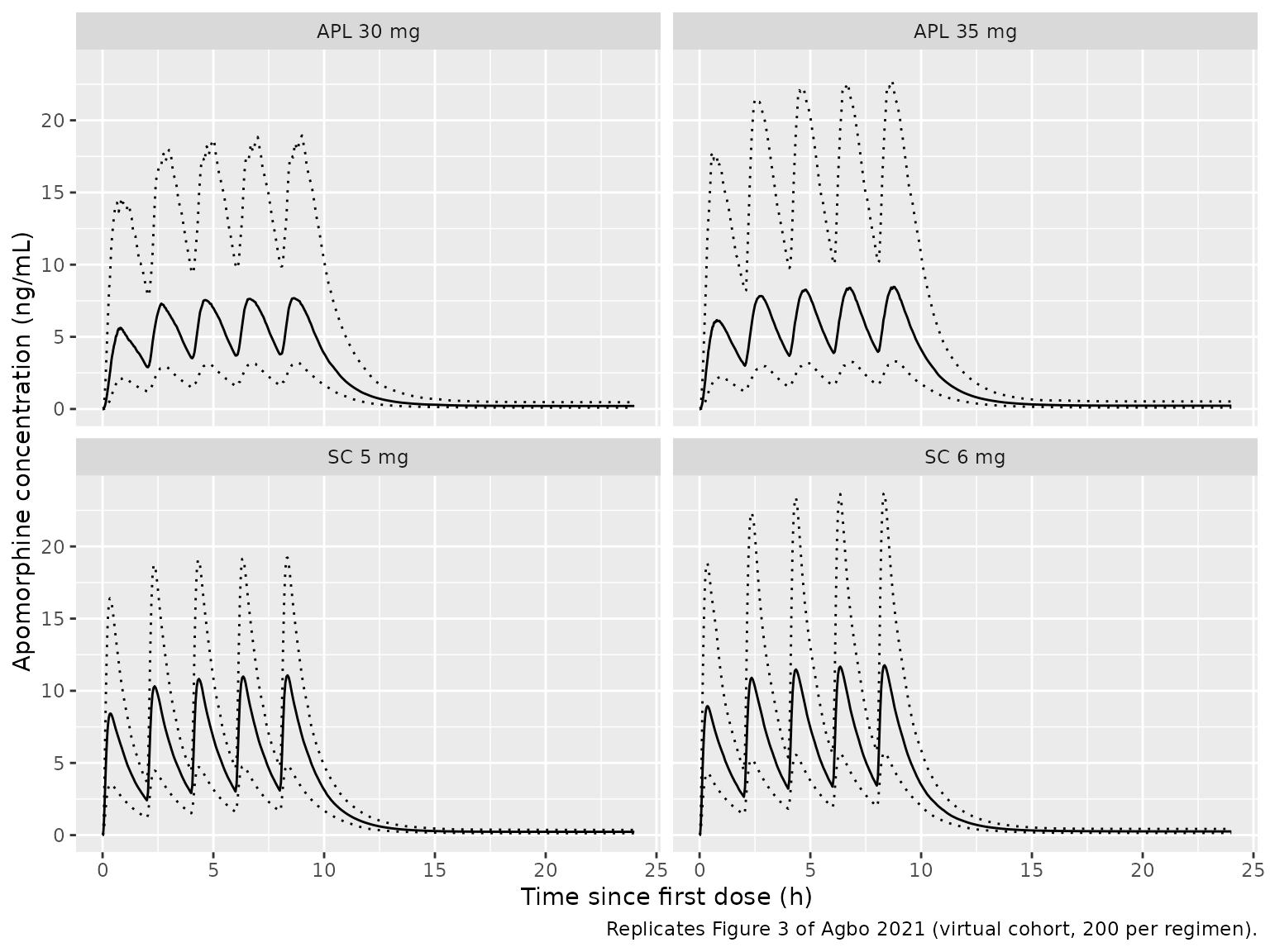
Figure 3 and the Results give the median predicted apomorphine exposure for 1000 simulated patients with PD after 30 or 35 mg sublingual film, or 5 or 6 mg subcutaneous apomorphine, every 2 hours for 5 doses: AUC0-24 66.7, 75.4, 66.7 and 80.0 ng*h/mL and Cmax about 9, 10, 10 and 12 ng/mL. The typical 78 kg patient reproduces these medians closely.
regimens <- tibble::tribble(
  ~treatment,     ~route, ~dose,
  "APL 30 mg",    "SL",   30,
  "APL 35 mg",    "SL",   35,
  "SC 5 mg",      "SC",    5,
  "SC 6 mg",      "SC",    6
)
ev_fig3_typ <- dplyr::bind_rows(lapply(seq_len(nrow(regimens)), function(i) {
  make_events(
    i, regimens$route[i], regimens$dose[i],
    wt = 78, n_dose = 5, treatment = regimens$treatment[i]
  )
}))
sim_fig3_typ <- solve_typ(ev_fig3_typ)
#> ℹ omega/sigma items treated as zero: 'etalcl', 'etalvc', 'etalvc_sulf', 'etalka', 'etalfdepot'
#> Warning: multi-subject simulation without without 'omega'
nca_fig3_typ <- nca_0_24(sim_fig3_typ, ev_fig3_typ, "Cc")

published_fig3 <- tibble::tribble(
  ~treatment,  ~cmax, ~auclast,
  "APL 30 mg",    9,     66.7,
  "APL 35 mg",   10,     75.4,
  "SC 5 mg",     10,     66.7,
  "SC 6 mg",     12,     80.0
)
knitr::kable(
  nlmixr2lib::ncaComparisonTable(
    simulated = nca_fig3_typ,
    reference = published_fig3,
    by = "treatment",
    units = c(cmax = "ng/mL", auclast = "ng*h/mL"),
    tolerance_pct = 20
  ),
  caption = paste(
    "Typical 78 kg patient with PD vs the paper's cohort medians",
    "(Figure 3; Results). Published Cmax values are the text's rounded",
    "approximations."
  )
)| NCA parameter | treatment | Reference | Simulated | % diff |
|---|---|---|---|---|
| Cmax (ng/mL) | APL 30 mg | 9 | 8.59 | -4.6% |
| Cmax (ng/mL) | APL 35 mg | 10 | 9.71 | -2.9% |
| Cmax (ng/mL) | SC 5 mg | 10 | 10.2 | +2.1% |
| Cmax (ng/mL) | SC 6 mg | 12 | 12.2 | +2.1% |
| AUClast (ng*h/mL) | APL 30 mg | 66.7 | 67.1 | +0.5% |
| AUClast (ng*h/mL) | APL 35 mg | 75.4 | 75.8 | +0.5% |
| AUClast (ng*h/mL) | SC 5 mg | 66.7 | 66.2 | -0.8% |
| AUClast (ng*h/mL) | SC 6 mg | 80 | 79.4 | -0.7% |
w3 <- nca_wide(nca_fig3_typ) |>
  dplyr::inner_join(published_fig3, by = "treatment", suffix = c("", "_pub"))
stopifnot(
  all(abs(w3$auclast / w3$auclast_pub - 1) < 0.05),
  all(abs(w3$cmax / w3$cmax_pub - 1) < 0.10)
)
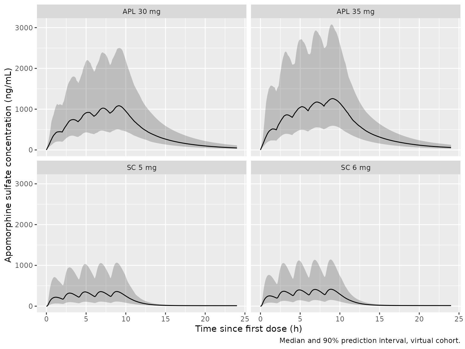
The paper also states that subcutaneous dosing gives apomorphine sulfate Cmax about 35% of that after sublingual dosing at the two comparative dose pairs. The sublingual excess comes from the swallowed fraction absorbed directly as the sulfate.
nca_sulf <- nca_wide(nca_0_24(sim_fig3_typ, ev_fig3_typ, "Cc_sulf"))
cmax_s <- stats::setNames(nca_sulf$cmax, nca_sulf$treatment)
sulf_ratio <- c(
  "SC 5 mg / APL 30 mg" = cmax_s[["SC 5 mg"]] / cmax_s[["APL 30 mg"]],
  "SC 6 mg / APL 35 mg" = cmax_s[["SC 6 mg"]] / cmax_s[["APL 35 mg"]]
)
sulf_ratio
#> SC 5 mg / APL 30 mg SC 6 mg / APL 35 mg
#>           0.3344612           0.3475605
stopifnot(all(abs(sulf_ratio - 0.35) < 0.05))
Virtual cohort
The paper simulated 1000 patients with PD by bootstrapping complete covariate vectors from the observed PD data. Those data are not public. The cohort below draws 200 patients per regimen. Weight is log-normal around the Table 2 PD mean (80 kg), with an assumed 20% CV, and draws are rejected and redrawn outside the observed PD range (50.7-146.1 kg). 31% are female (Table 2), all are outside study CTH-103, and every film has 3 min contact time (the Figure 2 typical value).
set.seed(20210401)
n_per_arm <- 200L

draw_wt <- function(n) {
  out <- numeric(0)
  while (length(out) < n) {
    x <- stats::rlnorm(n, meanlog = log(80) - 0.2^2 / 2, sdlog = 0.2)
    out <- c(out, x[x >= 50.7 & x <= 146.1])
  }
  out[seq_len(n)]
}

cohort_events <- dplyr::bind_rows(lapply(seq_len(nrow(regimens)), function(i) {
  wt <- draw_wt(n_per_arm)
  sexf <- stats::rbinom(n_per_arm, 1, 0.31)
  dplyr::bind_rows(lapply(seq_len(n_per_arm), function(j) {
    make_events(
      (i - 1L) * n_per_arm + j, regimens$route[i], regimens$dose[i],
      wt = wt[j], sexf = sexf[j], n_dose = 5,
      treatment = regimens$treatment[i]
    )
  }))
}))
stopifnot(
  !anyDuplicated(unique(cohort_events[, c("id", "time", "evid", "cmt")])),
  dplyr::n_distinct(cohort_events$id) == 4L * n_per_arm
)Replicate published figures
# Replicates Figure 3 of Agbo 2021: median and 90% prediction interval of
# apomorphine concentration, 5 doses every 2 h. Uses the individual
# prediction (no residual error), as the paper's exposure summaries do.
sim |>
  dplyr::filter(!is.na(Cc)) |>
  dplyr::group_by(treatment, time) |>
  dplyr::summarise(
    Q05 = stats::quantile(Cc, 0.05),
    Q50 = stats::quantile(Cc, 0.50),
    Q95 = stats::quantile(Cc, 0.95),
    .groups = "drop"
  ) |>
  ggplot(aes(time, Q50)) +
  geom_line(aes(y = Q05), linetype = "dotted") +
  geom_line(aes(y = Q95), linetype = "dotted") +
  geom_line() +
  facet_wrap(~treatment) +
  labs(
    x = "Time since first dose (h)",
    y = "Apomorphine concentration (ng/mL)",
    caption = "Replicates Figure 3 of Agbo 2021 (virtual cohort, 200 per regimen)."
  )
# Apomorphine sulfate under the same regimens (not plotted in the paper).
sim |>
  dplyr::filter(!is.na(Cc_sulf)) |>
  dplyr::group_by(treatment, time) |>
  dplyr::summarise(
    Q05 = stats::quantile(Cc_sulf, 0.05),
    Q50 = stats::quantile(Cc_sulf, 0.50),
    Q95 = stats::quantile(Cc_sulf, 0.95),
    .groups = "drop"
  ) |>
  ggplot(aes(time, Q50)) +
  geom_ribbon(aes(ymin = Q05, ymax = Q95), alpha = 0.25) +
  geom_line() +
  facet_wrap(~treatment) +
  labs(
    x = "Time since first dose (h)",
    y = "Apomorphine sulfate concentration (ng/mL)",
    caption = "Median and 90% prediction interval, virtual cohort."
  )
PKNCA validation
nca_cohort <- nca_0_24(sim, cohort_events, "Cc")
cmp_cohort <- nlmixr2lib::ncaComparisonTable(
  simulated = nca_cohort,
  reference = published_fig3,
  by = "treatment",
  units = c(cmax = "ng/mL", auclast = "ng*h/mL"),
  tolerance_pct = 20
)
knitr::kable(
  cmp_cohort,
  caption = paste(
    "Virtual-cohort medians (200 per regimen) vs the paper's medians of",
    "1000 bootstrapped patients with PD (Figure 3; Results). * differs by >20%."
  )
)| NCA parameter | treatment | Reference | Simulated | % diff |
|---|---|---|---|---|
| Cmax (ng/mL) | APL 30 mg | 9 | 7.99 | -11.2% |
| Cmax (ng/mL) | APL 35 mg | 10 | 8.86 | -11.4% |
| Cmax (ng/mL) | SC 5 mg | 10 | 11.1 | +10.7% |
| Cmax (ng/mL) | SC 6 mg | 12 | 11.8 | -1.9% |
| AUClast (ng*h/mL) | APL 30 mg | 66.7 | 60.9 | -8.6% |
| AUClast (ng*h/mL) | APL 35 mg | 75.4 | 66.8 | -11.4% |
| AUClast (ng*h/mL) | SC 5 mg | 66.7 | 69.1 | +3.5% |
| AUClast (ng*h/mL) | SC 6 mg | 80 | 76.4 | -4.6% |
wc <- nca_wide(nca_cohort) |>
  dplyr::inner_join(published_fig3, by = "treatment", suffix = c("", "_pub"))
stopifnot(
  # Centre only. The cohort's weight distribution is an assumption and each
  # median is over 200 subjects whose draw differs across rxode2 builds and
  # thread counts, so this is a coarse envelope; the structural check is the
  # deterministic typical-value gate above (within 1% on AUC0-24). Observed
  # while authoring: AUC0-24 -11.4% to +3.5%, Cmax -11.4% to +10.7%. A
  # mis-transcribed clearance, volume, bioavailability or unit moves these
  # by well over 25%.
  all(abs(wc$auclast / wc$auclast_pub - 1) < 0.25),
  all(abs(wc$cmax / wc$cmax_pub - 1) < 0.25)
)
The paper’s Table 4 gives individual predicted exposure after a single 10 mg film in the patients with PD: median Cmax 2.45 and 2.07 ng/mL and median AUC 5.34 and 5.31 ng*h/mL for normal renal function and mild renal impairment. The typical 78 kg patient with PD sits close to these medians:
ev_t4 <- make_events(1L, "SL", 10, wt = 78, treatment = "10 mg")
w_t4 <- nca_wide(nca_0_24(solve_typ(ev_t4), ev_t4, "Cc"))
#> ℹ omega/sigma items treated as zero: 'etalcl', 'etalvc', 'etalvc_sulf', 'etalka', 'etalfdepot'
w_t4
#> # A tibble: 1 × 3
#>   treatment auclast  cmax
#>   <chr>       <dbl> <dbl>
#> 1 10 mg        5.68  2.62
Assumptions and deviations
-
k23 = CL/V2with a weight-independent CL. Table 3 reports CL/F as the estimated parameter and puts the IIV onk23, “equal to CL/V2”. The model therefore computeskel = cl / vcfrom the individual V2/F, and thek23random effect is carried asetalcl. Underk23 = CL/V2 * exp(eta)that is exactly an eta on CL. The maintainers chose this over ak23that is itself weight-independent, in which clearance would grow with V2/F. This reading reproduces the Figure 3 AUC0-24 medians within 1% for a typical 78 kg patient and the Figure 2 Cmax values within about 1%; the alternative is 3-5% off on every one. It also agrees with the Discussion, which says apparent clearance is not influenced by weight. The control stream is not published, so it cannot be confirmed whether V2 in thek23denominator included the V2/F random effect. The typical-value checks cannot tell the two apart. -
“AUC0-inf” in the paper is a finite-window value.
With
k62 = 0.0048/h, about three quarters of the true AUC0-inf lies in a terminal phase with a half-life of several hundred hours at concentrations near 0.03 ng/mL. The paper’s “AUC0-inf” of 10.60 ngh/mL for the typical patient is close to the model’s AUC0-24 (9.9 ngh/mL) and far from the model’s true AUC0-inf (about 45 ng*h/mL). This vignette therefore compares against PKNCA AUC0-24. The paper’s exact NCA window and extrapolation are not reported; the remaining 7-10% gap on these two AUCs is not otherwise explained. Cmax, the body-weight AUC ratio and all Figure 3 values agree. -
Residual error. Methods Eq. 3 introduces a
log-transformed error model; the Results state that a proportional
residual error model was used for both analytes. Both are encoded as
proportional (
prop()) with SD 0.443 and 0.580, the Table 3 percentages read as fractions. -
IIV on F1 multiplies the whole sublingual
bioavailability
Biosl * Biorsc * dose effect(log-normal, Methods Eq. 1). The swallowed fractionF5 = 1 - Bioslcarries no IIV, because Table 3 lists none for it. -
Categorical covariates (study CTH-103 on V2/F,
female sex on V3/F) use the
1 + theta * Xform of Methods Eq. 5. The Results describe both as “the proportional shift from the reference condition”, and the negative estimates match Eq. 5’s constraint thattheta > -1. -
Apomorphine sulfate units. Amounts move 1:1 from
apomorphine to the sulfate compartment, with no molecular-weight
conversion. V3/F (1.42 L) is an apparent volume estimated against the
sulfate data, so
Cc_sulfis in the units of the fitted observations (ng/mL, as for all concentrations in the paper). The supplementary goodness-of-fit and VPC figures (S1-S3), which would show the sulfate concentration scale, were not included in the open access deposit. The published SC/sublingual sulfate Cmax ratio (about 35%) is reproduced. -
Contact time and dose covariates are per
administration. The sublingual-only covariates
DUR_SL_CONTACTandDOSE_APOMORPHINE_SL_MGmust be present on every row but only affect the sublingual chain. Their value on subcutaneous records is irrelevant. - Virtual cohort. The PD weight distribution (log-normal, mean 80 kg, 20% CV, truncated to the observed range) is an assumption, because the paper bootstrapped its own PD covariate data. All subjects use a 3 min contact time and are outside study CTH-103. The Figure 3 comparison is gated on medians only.
-
Not reproduced. The Figure 2 forest plot’s dose
rows come from a simulation with parameter uncertainty and do not equal
(dose/20)^-0.206exactly (for example 1.18 at 10 mg vs 1.15 from the point estimate). The point estimate is used here. The Discussion’s 30-vs-10 mg claim (80%) is reproduced exactly. - No erratum or correction notice was found for this article (EuropePMC, checked 2026-09-28).