Levofloxacin and moxifloxacin in MDR-TB (Sidamo 2022)
Source:vignettes/articles/Sidamo_2022_fluoroquinolones_mdr_tb.Rmd
Sidamo_2022_fluoroquinolones_mdr_tb.RmdModel and source
Sidamo 2022 fitted two separate one-compartment population PK models, one for levofloxacin and one for moxifloxacin, to steady-state plasma concentrations from Ethiopian adults treated for multidrug- or rifampicin-resistant tuberculosis. Both are packaged:
-
Sidamo_2022_levofloxacin: One-compartment population pharmacokinetic model with first-order absorption, an absorption lag time and linear elimination for oral levofloxacin in Ethiopian adults with multidrug- or rifampicin-resistant tuberculosis (Sidamo 2022). Serum creatinine is retained as a power covariate on CL/F, but its exponent is not reported and is carried as fixed(0); the combined additive and proportional residual-error magnitudes are not reported and are carried as fixed(0). -
Sidamo_2022_moxifloxacin: One-compartment population pharmacokinetic model with first-order absorption and linear elimination for oral moxifloxacin in Ethiopian adults with multidrug- or rifampicin-resistant tuberculosis (Sidamo 2022). Body mass index is retained as a power covariate on V/F, but its exponent is not reported and is carried as fixed(0); the additive residual-error magnitude is not reported and is carried as fixed(0). - Citation: Sidamo T, Rao PS, Aklillu E, Shibeshi W, Park Y, Cho YS, Shin JG, Heysell SK, Mpagama SG, Engidawork E. Population Pharmacokinetics of Levofloxacin and Moxifloxacin, and the Probability of Target Attainment in Ethiopian Patients with Multidrug-Resistant Tuberculosis. Infect Drug Resist. 2022;15:6839-6852. doi:10.2147/IDR.S389442
- Article (open access): https://doi.org/10.2147/IDR.S389442
Population
The study (Methods, Results and Table 1) followed outpatients with MDR/RR-TB at four hospitals in Southern Ethiopia. Patients were 18 years or older, with or without HIV co-infection, and had received a levofloxacin-based regimen (750 or 1000 mg/day) or a moxifloxacin-based regimen (600 mg/day) for at least 8 days. Severely ill and anaemic patients (haematocrit below 25%) were excluded. Plasma was sampled pre-dose and at 2, 4, 6, 9, 12 and 24 h after a directly observed dose taken after breakfast. Of 55 sampled patients, 39 had acceptable profiles: 21 on levofloxacin and 18 on moxifloxacin.
| Characteristic (Table 1) | Levofloxacin (n = 21) | Moxifloxacin (n = 18) |
|---|---|---|
| Age, years | 26 (20-30) | 26 (20-37) |
| Male, n (%) | 12 (57.1) | 8 (44.4) |
| Weight, kg | 45 (42.5-52.3) | 51 (46.6-65.0) |
| BMI, kg/m^2 | 16.7 (15.6-18) | 17.3 (16.2-19.2) |
| Malnourished (BMI < 16), n (%) | 9 (42.9) | 10 (55.6) |
| Serum creatinine, mg/dL | 1 (0.8-1.3) | 1 (0.8-1.4) |
Values are median (IQR) unless stated. The same information is available programmatically:
str(readModelDb("Sidamo_2022_levofloxacin")()$population, give.attr = FALSE)
#> List of 15
#>  $ species       : chr "human"
#>  $ n_subjects    : int 21
#>  $ n_studies     : int 1
#>  $ age_range     : chr "adults 18 years and older (median 26 years, IQR 20-30)"
#>  $ age_median    : chr "26 years"
#>  $ weight_range  : chr "IQR 42.5-52.3 kg"
#>  $ weight_median : chr "45 kg"
#>  $ bmi_median    : chr "16.7 kg/m^2 (IQR 15.6-18)"
#>  $ sex_female_pct: num 42.9
#>  $ race_ethnicity: chr "Ethiopian"
#>  $ disease_state : chr "Multidrug- or rifampicin-resistant pulmonary tuberculosis (MDR/RR-TB) outpatients, with or without HIV co-infec"| __truncated__
#>  $ dose_range    : chr "Levofloxacin 750 or 1000 mg orally once daily for at least 8 days before PK sampling (steady state)."
#>  $ regions       : chr "Southern Ethiopia (Butajira, Yirgalem, Arbaminch and Nigist Eleni Mohammed Memorial hospitals)."
#>  $ renal_function: chr "Serum creatinine median 1 mg/dL (IQR 0.8-1.3)."
#>  $ notes         : chr "39 of 55 sampled patients had acceptable profiles (21 levofloxacin, 18 moxifloxacin). Plasma sampled pre-dose a"| __truncated__
Source trace
Both models are one-compartment with first-order absorption and linear elimination, fitted in Phoenix NLME with first-order conditional estimation. The levofloxacin model has an absorption lag time and a combined additive and proportional residual error. The moxifloxacin model has no lag time and an additive residual error (Results, ‘The Population PK Model’). All parameters are apparent oral values.
| Equation / parameter | Levofloxacin | Moxifloxacin | Source location |
|---|---|---|---|
lka (ka, 1/h) |
log(0.2) | log(0.5) | Table 2, ‘GM (%RSE)’ |
lvc (V/F, L) |
log(122) | log(102.2) | Table 2 |
lcl (CL/F, L/h) |
log(10.4) | log(20) | Table 2 |
ltlag (Tlag, h) |
log(0.2) | – | Table 2 |
| Covariate centring value | CREAT 1.1 mg/dL on CL/F | BMI 17.8 kg/m^2 on V/F | Table 2, ‘Cr (mg/dL)’ and ‘BMI (Kg.m2)’ rows; see Reading Table 2 |
e_creat_cl, e_bmi_vc (power
exponents) |
fixed(0) | fixed(0) | Not reported; Methods Equation 1 gives the power form |
etalka (variance) |
0.01941 (14 %CV) | 0.2987 (59 %CV) | Table 2, ‘%CV (Shrinkage, %)’, as log(1 + CV^2) |
etalvc (variance) |
0.065413 (26 %CV) | 0.0099503 (10 %CV) | Table 2 |
etalcl (variance) |
0.36158 (66 %CV) | 0.00072873 (2.7 %CV) | Table 2 |
etaltlag (variance) |
0.0011553 (3.4 %CV) | – | Table 2 |
propSd, addSd
|
fixed(0), fixed(0) | –, fixed(0) | Error models named in Results; magnitudes not reported |
(COV / COVmean)^theta2 |
CL/F | V/F | Methods Equation 1 |
exp(theta + eta) |
– | – | Methods Equation 3, exponential IIV |
d/dt(depot), d/dt(central),
alag(depot)
|
– | – | Results: one-compartment, first-order absorption, lag for levofloxacin only |
Reading Table 2
Results state that serum creatinine was retained on levofloxacin
clearance and BMI on moxifloxacin volume. Methods Equation 1 gives the
form, TVP = theta1 * (COV / COVmean)^theta2. Table 2 prints
a single number for each covariate in the ‘GM (%RSE)’ column: ‘Cr
(mg/dL) 1.1 (10)’ and ‘BMI (Kg.m2) 17.8 (1.1)’. It does not say whether
that number is the exponent theta2 or the centring value COVmean.
The packaged models read it as COVmean, with the exponent unreported:
- Both rows carry the covariate’s units, which a dimensionless exponent would not.
- Both values match the cohort’s mean covariate. Levofloxacin creatinine has a median of 1 mg/dL and a right-skewed IQR of 0.8-1.3, so its mean is near 1.1. Moxifloxacin BMI has a median of 17.3 kg/m^2 and an IQR of 16.2-19.2, so its mean is near 17.8.
- An exponent of 17.8 on BMI is not physically meaningful. It would cut V/F by 60% between the median BMI and the centring BMI, a difference of only 0.5 kg/m^2. A single reading must hold for both rows, and only the COVmean reading does.
- The same group’s earlier Phoenix analysis (Rao 2021, packaged as
Rao_2021_pyrazinamideandRao_2021_ethambutol) also left its covariate coefficients unprinted.
The exponents are therefore fixed(0) placeholders. The
covariate columns stay in the model, so the structure is the published
one, but CREAT and BMI have no effect until
the coefficients are known. The ‘%CV’ column also prints values for both
covariate rows, 14.7 and 4.5, each with shrinkage ‘NA’. As exponents,
14.7 on creatinine would be as implausible as 17.8 on BMI. A
residual-error reading does not fit either. Neither value is used.
Virtual cohort and simulation
The paper simulated each patient’s own profile at 750, 1000 and 1500
mg of levofloxacin and 600, 800 and 1000 mg of moxifloxacin (Methods,
‘Drug Exposure’). The virtual cohort here is 100 subjects per dose. Each
subject gets 8 once-daily doses into depot, and
central is observed every 0.5 h over the last dosing
interval (168-192 h), which is at steady state for both drugs.
Creatinine and BMI are drawn log-normally to match the Table 1 median
and IQR of each drug’s cohort. With the exponents at zero they do not
change the simulation, but they keep the covariate path exercised.
doses <- list(
  levofloxacin = c(750, 1000, 1500),
  moxifloxacin = c(600, 800, 1000)
)
n_per_arm <- 100L
obs_times <- seq(168, 192, by = 0.5)

# Log-normal draw matching a published median and IQR.
draw_lognormal <- function(n, median, q1, q3) {
  exp(rnorm(n, log(median), log(q3 / q1) / (2 * qnorm(0.75))))
}

make_arm <- function(drug, dose, id_offset) {
  ids <- id_offset + seq_len(n_per_arm)
  covs <- tibble(
    id = ids,
    CREAT = draw_lognormal(n_per_arm, 1, 0.8, if (drug == "levofloxacin") 1.3 else 1.4),
    BMI = if (drug == "levofloxacin") {
      draw_lognormal(n_per_arm, 16.7, 15.6, 18)
    } else {
      draw_lognormal(n_per_arm, 17.3, 16.2, 19.2)
    }
  )
  dose_rows <- tidyr::expand_grid(id = ids, time = seq(0, 168, by = 24)) |>
    mutate(amt = dose, evid = 1L, cmt = "depot")
  obs_rows <- tidyr::expand_grid(id = ids, time = obs_times) |>
    mutate(amt = 0, evid = 0L, cmt = "central")
  bind_rows(dose_rows, obs_rows) |>
    left_join(covs, by = "id") |>
    mutate(drug = drug, treatment = paste(dose, "mg")) |>
    arrange(id, time, desc(evid))
}

rxode2::rxSetSeed(20221201)
events <- list()
for (drug in names(doses)) {
  arms <- lapply(seq_along(doses[[drug]]), function(i) {
    make_arm(drug, doses[[drug]][i], id_offset = (i - 1L) * n_per_arm)
  })
  events[[drug]] <- bind_rows(arms)
  stopifnot(!anyDuplicated(events[[drug]][, c("id", "time", "evid")]))
}
mods <- list(
  levofloxacin = readModelDb("Sidamo_2022_levofloxacin"),
  moxifloxacin = readModelDb("Sidamo_2022_moxifloxacin")
)
sim <- bind_rows(lapply(names(mods), function(drug) {
  as.data.frame(rxode2::rxSolve(
    mods[[drug]],
    events = events[[drug]],
    keep = c("drug", "treatment")
  ))
}))
#> ℹ parameter labels from comments will be replaced by 'label()'
#> ℹ parameter labels from comments will be replaced by 'label()'
stopifnot(!anyNA(sim$Cc))
sim |>
  mutate(tad = time - 168) |>
  group_by(drug, treatment, tad) |>
  summarise(
    q05 = quantile(Cc, 0.05), q50 = median(Cc), q95 = quantile(Cc, 0.95),
    .groups = "drop"
  ) |>
  ggplot(aes(tad, q50, colour = treatment, fill = treatment)) +
  geom_ribbon(aes(ymin = q05, ymax = q95), alpha = 0.15, colour = NA) +
  geom_line() +
  facet_wrap(~drug, scales = "free_y") +
  labs(
    x = "Time after dose at steady state (h)", y = "Plasma concentration (mg/L)",
    colour = "Dose", fill = "Dose",
    caption = "Median and 90% interval of 100 simulated subjects per dose (between-subject variability only)."
  ) +
  theme_bw()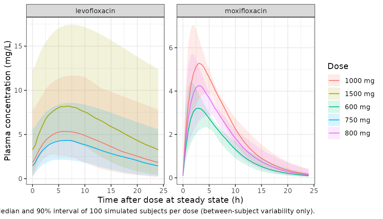
Typical-value comparison with Table 3
Table 3 gives the median Cmax and AUC0-24 at each dose, simulated from the patients’ individual estimates, alongside the observed non-compartmental values at the doses actually given. The paper does not say whether its simulations are single-dose or steady-state, so the typical-value models are solved both ways.
published_t3 <- tibble::tribble(
  ~drug, ~dose, ~source, ~cmax, ~auc24,
  "levofloxacin", 750, "simulated", 7.5, 60.9,
  "levofloxacin", 1000, "simulated", 10.0, 81.5,
  "levofloxacin", 1500, "simulated", 15.1, 122.7,
  "levofloxacin", 750, "observed", 5.3, 58.1,
  "levofloxacin", 1000, "observed", 7.4, 103.4,
  "moxifloxacin", 600, "simulated", 2.6, 25.1,
  "moxifloxacin", 800, "simulated", 3.5, 33.4,
  "moxifloxacin", 1000, "simulated", 4.4, 41.8,
  "moxifloxacin", 600, "observed", 3.2, 28.2
)

trap_auc <- function(time, conc) {
  sum(diff(time) * (head(conc, -1) + tail(conc, -1)) / 2)
}

typical_profile <- function(drug, dose, steady_state = FALSE) {
  ev <- if (steady_state) {
    rxode2::et(amt = dose, cmt = "depot", ii = 24, addl = 29) |>
      rxode2::et(seq(696, 720, by = 0.05), cmt = "central")
  } else {
    rxode2::et(amt = dose, cmt = "depot") |>
      rxode2::et(seq(0, 24, by = 0.05), cmt = "central")
  }
  ev <- as.data.frame(ev)
  ev$CREAT <- 1.1
  ev$BMI <- 17.8
  s <- as.data.frame(rxode2::rxSolve(rxode2::zeroRe(mods[[drug]]), events = ev))
  tibble(cmax = max(s$Cc), auc24 = trap_auc(s$time, s$Cc))
}

typical <- published_t3 |>
  rowwise() |>
  mutate(
    sd = list(typical_profile(drug, dose)),
    ss = list(typical_profile(drug, dose, steady_state = TRUE))
  ) |>
  ungroup() |>
  mutate(
    cmax_sd = sapply(sd, `[[`, "cmax"),
    auc_sd = sapply(sd, `[[`, "auc24"),
    cmax_ss = sapply(ss, `[[`, "cmax"),
    auc_ss = sapply(ss, `[[`, "auc24"),
    pct_cmax_ss = 100 * (cmax_ss - cmax) / cmax,
    pct_auc_sd = 100 * (auc_sd - auc24) / auc24,
    pct_auc_ss = 100 * (auc_ss - auc24) / auc24
  )
#> ℹ parameter labels from comments will be replaced by 'label()'
#> ℹ omega/sigma items treated as zero: 'etalka', 'etalvc', 'etalcl', 'etaltlag'
#> ℹ parameter labels from comments will be replaced by 'label()'
#> ℹ omega/sigma items treated as zero: 'etalka', 'etalvc', 'etalcl', 'etaltlag'
#> ℹ parameter labels from comments will be replaced by 'label()'
#> ℹ omega/sigma items treated as zero: 'etalka', 'etalvc', 'etalcl', 'etaltlag'
#> ℹ parameter labels from comments will be replaced by 'label()'
#> ℹ omega/sigma items treated as zero: 'etalka', 'etalvc', 'etalcl', 'etaltlag'
#> ℹ parameter labels from comments will be replaced by 'label()'
#> ℹ omega/sigma items treated as zero: 'etalka', 'etalvc', 'etalcl', 'etaltlag'
#> ℹ parameter labels from comments will be replaced by 'label()'
#> ℹ omega/sigma items treated as zero: 'etalka', 'etalvc', 'etalcl'
#> ℹ parameter labels from comments will be replaced by 'label()'
#> ℹ omega/sigma items treated as zero: 'etalka', 'etalvc', 'etalcl'
#> ℹ parameter labels from comments will be replaced by 'label()'
#> ℹ omega/sigma items treated as zero: 'etalka', 'etalvc', 'etalcl'
#> ℹ parameter labels from comments will be replaced by 'label()'
#> ℹ omega/sigma items treated as zero: 'etalka', 'etalvc', 'etalcl'
#> ℹ parameter labels from comments will be replaced by 'label()'
#> ℹ omega/sigma items treated as zero: 'etalka', 'etalvc', 'etalcl', 'etaltlag'
#> ℹ parameter labels from comments will be replaced by 'label()'
#> ℹ omega/sigma items treated as zero: 'etalka', 'etalvc', 'etalcl', 'etaltlag'
#> ℹ parameter labels from comments will be replaced by 'label()'
#> ℹ omega/sigma items treated as zero: 'etalka', 'etalvc', 'etalcl', 'etaltlag'
#> ℹ parameter labels from comments will be replaced by 'label()'
#> ℹ omega/sigma items treated as zero: 'etalka', 'etalvc', 'etalcl', 'etaltlag'
#> ℹ parameter labels from comments will be replaced by 'label()'
#> ℹ omega/sigma items treated as zero: 'etalka', 'etalvc', 'etalcl', 'etaltlag'
#> ℹ parameter labels from comments will be replaced by 'label()'
#> ℹ omega/sigma items treated as zero: 'etalka', 'etalvc', 'etalcl'
#> ℹ parameter labels from comments will be replaced by 'label()'
#> ℹ omega/sigma items treated as zero: 'etalka', 'etalvc', 'etalcl'
#> ℹ parameter labels from comments will be replaced by 'label()'
#> ℹ omega/sigma items treated as zero: 'etalka', 'etalvc', 'etalcl'
#> ℹ parameter labels from comments will be replaced by 'label()'
#> ℹ omega/sigma items treated as zero: 'etalka', 'etalvc', 'etalcl'

typical |>
  select(drug, dose, source, cmax, cmax_sd, cmax_ss, auc24, auc_sd, auc_ss, pct_cmax_ss, pct_auc_ss) |>
  dplyr::rename(
    "Drug" = drug,
    "Dose (mg)" = dose,
    "Table 3 row" = source,
    "Table 3 Cmax" = cmax,
    "Typical single-dose Cmax" = cmax_sd,
    "Typical steady-state Cmax" = cmax_ss,
    "Table 3 AUC0-24" = auc24,
    "Typical single-dose AUC0-24" = auc_sd,
    "Typical steady-state AUC0-24" = auc_ss,
    "Cmax % diff (steady state)" = pct_cmax_ss,
    "AUC % diff (steady state)" = pct_auc_ss
  ) |>
  knitr::kable(
    digits = 1,
    caption = "Typical-value Cmax (mg/L) and AUC0-24 (mg*h/L) at the covariate centring values, against the Table 3 medians of Sidamo 2022."
)| Drug | Dose (mg) | Table 3 row | Table 3 Cmax | Typical single-dose Cmax | Typical steady-state Cmax | Table 3 AUC0-24 | Typical single-dose AUC0-24 | Typical steady-state AUC0-24 | Cmax % diff (steady state) | AUC % diff (steady state) |
|---|---|---|---|---|---|---|---|---|---|---|
| levofloxacin | 750 | simulated | 7.5 | 3.3 | 4.1 | 60.9 | 56.0 | 72.1 | -45.0 | 18.4 |
| levofloxacin | 1000 | simulated | 10.0 | 4.4 | 5.5 | 81.5 | 74.7 | 96.2 | -45.0 | 18.0 |
| levofloxacin | 1500 | simulated | 15.1 | 6.5 | 8.3 | 122.7 | 112.1 | 144.2 | -45.3 | 17.5 |
| levofloxacin | 750 | observed | 5.3 | 3.3 | 4.1 | 58.1 | 56.0 | 72.1 | -22.1 | 24.1 |
| levofloxacin | 1000 | observed | 7.4 | 4.4 | 5.5 | 103.4 | 74.7 | 96.2 | -25.6 | -7.0 |
| moxifloxacin | 600 | simulated | 2.6 | 3.2 | 3.3 | 25.1 | 29.5 | 30.0 | 25.4 | 19.5 |
| moxifloxacin | 800 | simulated | 3.5 | 4.3 | 4.3 | 33.4 | 39.4 | 40.0 | 24.2 | 19.8 |
| moxifloxacin | 1000 | simulated | 4.4 | 5.4 | 5.4 | 41.8 | 49.2 | 50.0 | 23.5 | 19.6 |
| moxifloxacin | 600 | observed | 3.2 | 3.2 | 3.3 | 28.2 | 29.5 | 30.0 | 1.9 | 6.4 |
lfx <- typical[typical$drug == "levofloxacin", ]
mxf <- typical[typical$drug == "moxifloxacin", ]
mxf_obs <- mxf[mxf$source == "observed", ]
lfx_sim <- lfx[lfx$source == "simulated", ]
stopifnot(
  # Moxifloxacin: the steady-state typical value reproduces the observed
  # median Cmax and AUC0-24 at 600 mg (realised +2% and +6%). A
  # mis-transcribed CL or V moves these by tens of percent.
  abs(mxf_obs$pct_cmax_ss) < 15,
  abs(mxf_obs$pct_auc_ss) < 15,
  # Levofloxacin: the Table 3 simulated AUC0-24 medians lie between the
  # single-dose and steady-state typical values at every dose, and stay
  # dose-proportional, as the linear model requires.
  all(lfx_sim$auc_sd < lfx_sim$auc24 & lfx_sim$auc24 < lfx_sim$auc_ss),
  abs(lfx_sim$auc24[3] / lfx_sim$auc24[1] - 2) < 0.05
)
These are deterministic solves with no random draw, so the bounds above are tight on purpose.
The moxifloxacin model reproduces the observed steady-state exposure at 600 mg. Its simulated rows in Table 3 run about 15-20% below the typical value, and the Table 3 means (31.5, 40.6 and 50.8 mg*h/L) are within 5% of it.
For levofloxacin, the AUC0-24 medians lie between the single-dose and steady-state solves. The Table 3 Cmax values do not. The simulated medians (7.5, 10.0 and 15.1 mg/L) are about 1.8 times the steady-state typical value, and even the observed medians (5.3 and 7.4 mg/L) are about 30% above it. With ka = 0.2 1/h and V/F = 122 L, the model’s ratio of Cmax to AUC0-24 at steady state is about 0.057 1/h. The simulated rows of Table 3 imply 0.12 1/h and the observed rows 0.07-0.09 1/h. Rounding ka to one decimal place cannot account for this, because even instant absorption limits the ratio to about 0.098 1/h at V/F = 122 L. The model is kept as published. The Assumptions section records the gap.
PKNCA comparison against Table 3
sim_nca <- sim |>
  dplyr::filter(!is.na(Cc)) |>
  dplyr::mutate(group = paste(drug, treatment)) |>
  dplyr::select(id, time, Cc, drug, treatment, group)

dose_df <- bind_rows(events) |>
  dplyr::filter(evid == 1) |>
  dplyr::mutate(group = paste(drug, treatment)) |>
  dplyr::select(id, time, amt, drug, treatment, group)

conc_obj <- PKNCA::PKNCAconc(
  sim_nca, Cc ~ time | group + id,
  concu = "mg/L", timeu = "h"
)
dose_obj <- PKNCA::PKNCAdose(
  dose_df, amt ~ time | group + id,
  doseu = "mg"
)
intervals <- data.frame(start = 168, end = 192, cmax = TRUE, tmax = TRUE, auclast = TRUE)
nca_res <- PKNCA::pk.nca(PKNCA::PKNCAdata(conc_obj, dose_obj, intervals = intervals))

per_subject <- as.data.frame(nca_res$result) |>
  dplyr::filter(PPTESTCD %in% c("cmax", "auclast")) |>
  dplyr::select(group, id, PPTESTCD, PPORRES) |>
  tidyr::pivot_wider(names_from = PPTESTCD, values_from = PPORRES) |>
  dplyr::left_join(
    dplyr::distinct(dose_df, group, drug, treatment, amt),
    by = "group"
  )
reference <- published_t3 |>
  dplyr::filter(source == "simulated") |>
  dplyr::mutate(group = paste(drug, paste(dose, "mg"))) |>
  dplyr::select(group, cmax, auclast = auc24)

cmp <- nlmixr2lib::ncaComparisonTable(
  simulated = nca_res,
  reference = reference,
  by = "group",
  params = c("cmax", "auclast"),
  units = c(cmax = "mg/L", auclast = "mg*h/L"),
  tolerance_pct = 20
)
knitr::kable(
  cmp,
  caption = "Simulated steady state (100 subjects per dose) vs. the Sidamo 2022 Table 3 simulated medians. * differs from the reference by >20%."
)| NCA parameter | group | Reference | Simulated | % diff |
|---|---|---|---|---|
| Cmax (mg/L) | levofloxacin 750 mg | 7.5 | 4.37 | -41.7%* |
| Cmax (mg/L) | levofloxacin 1000 mg | 10 | 5.38 | -46.2%* |
| Cmax (mg/L) | levofloxacin 1500 mg | 15.1 | 8.24 | -45.4%* |
| Cmax (mg/L) | moxifloxacin 600 mg | 2.6 | 3.21 | +23.6%* |
| Cmax (mg/L) | moxifloxacin 800 mg | 3.5 | 4.25 | +21.5%* |
| Cmax (mg/L) | moxifloxacin 1000 mg | 4.4 | 5.3 | +20.6%* |
| AUClast (mg*h/L) | levofloxacin 750 mg | 60.9 | 71.4 | +17.3% |
| AUClast (mg*h/L) | levofloxacin 1000 mg | 81.5 | 92.4 | +13.3% |
| AUClast (mg*h/L) | levofloxacin 1500 mg | 123 | 144 | +17.2% |
| AUClast (mg*h/L) | moxifloxacin 600 mg | 25.1 | 29.7 | +18.3% |
| AUClast (mg*h/L) | moxifloxacin 800 mg | 33.4 | 40.1 | +20.0%* |
| AUClast (mg*h/L) | moxifloxacin 1000 mg | 41.8 | 49.7 | +18.9% |
chk <- per_subject |>
  dplyr::group_by(drug, amt) |>
  dplyr::summarise(auclast = median(auclast), .groups = "drop") |>
  dplyr::inner_join(
    dplyr::filter(published_t3, source == "simulated"),
    by = c("drug", "amt" = "dose")
  ) |>
  dplyr::mutate(pct_auc = 100 * (auclast - auc24) / auc24)
stopifnot(
  # Centre, not extremes: the median over the three doses of each drug. The
  # expected offsets are about +18% (levofloxacin) and +20% (moxifloxacin),
  # where the Table 3 medians summarise shrunken individual estimates. A wrong
  # dose, unit or clearance moves every dose together, by far more.
  abs(median(chk$pct_auc[chk$drug == "levofloxacin"])) < 35,
  abs(median(chk$pct_auc[chk$drug == "moxifloxacin"])) < 35
)
The starred Cmax rows for levofloxacin repeat the typical-value gap above. The AUC0-24 medians are about 15-20% above Table 3 for both drugs. This is the size of offset expected when one median comes from a full-variability simulation and the other from 18-21 shrunken individual estimates.
Spread of AUC0-24
AUC0-24 at steady state is dose / CL, whatever the volume and absorption, so its spread across subjects reflects between-subject variability in CL alone. The Table 3 values come from the patients’ own estimates, which shrinkage pulls toward the typical value. Their spread should therefore be no wider than that of a simulation with the full between-subject variances.
iqr_ratio <- function(x) unname(quantile(x, 0.75) / quantile(x, 0.25))
spread <- per_subject |>
  dplyr::filter(amt %in% c(750, 600)) |>
  dplyr::group_by(drug, amt) |>
  dplyr::summarise(sim_iqr_ratio = iqr_ratio(auclast), .groups = "drop") |>
  dplyr::mutate(
    table3_iqr_ratio = ifelse(drug == "levofloxacin", 81.8 / 40.0, 47.0 / 19.0)
  )
spread |>
  dplyr::rename(
    "Drug" = drug,
    "Dose (mg)" = amt,
    "Simulated AUC0-24 Q3/Q1" = sim_iqr_ratio,
    "Table 3 simulated AUC0-24 Q3/Q1" = table3_iqr_ratio
  ) |>
knitr::kable(digits = 2)| Drug | Dose (mg) | Simulated AUC0-24 Q3/Q1 | Table 3 simulated AUC0-24 Q3/Q1 |
|---|---|---|---|
| levofloxacin | 750 | 2.50 | 2.04 |
| moxifloxacin | 600 | 1.04 | 2.47 |
For levofloxacin the full-variability spread (66% CV on CL) is at least as wide as Table 3’s, as it should be. For moxifloxacin it is not. The printed 2.7% CV on CL gives an AUC0-24 interquartile ratio near 1.0, while Table 3 shows about 2.5 for the simulated rows and 2.6 (19.3-50.8 mgh/L) for the observed NCA at 600 mg. The Discussion also reports individual 600 mg AUC0-24 values from 3.5 to 72.2 mgh/L. None of the other variability entries in the moxifloxacin rows of Table 2 would be wide enough to explain this if moved to CL. The moxifloxacin model therefore reproduces the typical exposure but understates its between-subject spread; see Assumptions.
Probability of target attainment
Figures 4 and 5 report the percentage of patients whose AUC0-24/MIC reaches the kill target (146 for levofloxacin, 53 for moxifloxacin) or the resistance-suppression target (360 and 100). The values below are those quoted in the Results text. A dash means the text gives no number.
pta_pub <- tibble::tribble(
  ~drug, ~amt, ~mic, ~target, ~published,
  "levofloxacin", 750, 0.5, 146, 29,
  "levofloxacin", 1000, 0.5, 146, 62,
  "levofloxacin", 1500, 0.5, 146, 95,
  "levofloxacin", 750, 0.5, 360, 0,
  "levofloxacin", 1000, 0.5, 360, 0,
  "levofloxacin", 1500, 0.5, 360, 4.8,
  "levofloxacin", 1500, 1, 146, 24,
  "moxifloxacin", 600, 0.25, 53, 94.4,
  "moxifloxacin", 800, 0.25, 53, 94.4,
  "moxifloxacin", 1000, 0.25, 53, 94.4,
  "moxifloxacin", 600, 0.25, 100, 50,
  "moxifloxacin", 800, 0.25, 100, 77.8,
  "moxifloxacin", 1000, 0.25, 100, 94.4,
  "moxifloxacin", 600, 1, 53, 11.1,
  "moxifloxacin", 800, 1, 53, 27.8,
  "moxifloxacin", 1000, 1, 53, 38.9
)

pta <- pta_pub |>
  dplyr::left_join(per_subject, by = c("drug", "amt"), relationship = "many-to-many") |>
  dplyr::group_by(drug, amt, mic, target, published) |>
  dplyr::summarise(simulated = 100 * mean(auclast / mic >= target), .groups = "drop")

pta |>
  dplyr::rename(
    "Drug" = drug,
    "Dose (mg)" = amt,
    "MIC (mg/L)" = mic,
    "AUC0-24/MIC target" = target,
    "Published PTA (%)" = published,
    "Simulated PTA (%)" = simulated
  ) |>
knitr::kable(digits = c(0, 0, 2, 0, 1, 1))| Drug | Dose (mg) | MIC (mg/L) | AUC0-24/MIC target | Published PTA (%) | Simulated PTA (%) |
|---|---|---|---|---|---|
| levofloxacin | 750 | 0.50 | 146 | 29.0 | 50 |
| levofloxacin | 750 | 0.50 | 360 | 0.0 | 5 |
| levofloxacin | 1000 | 0.50 | 146 | 62.0 | 62 |
| levofloxacin | 1000 | 0.50 | 360 | 0.0 | 15 |
| levofloxacin | 1500 | 0.50 | 146 | 95.0 | 85 |
| levofloxacin | 1500 | 0.50 | 360 | 4.8 | 30 |
| levofloxacin | 1500 | 1.00 | 146 | 24.0 | 49 |
| moxifloxacin | 600 | 0.25 | 53 | 94.4 | 100 |
| moxifloxacin | 600 | 0.25 | 100 | 50.0 | 100 |
| moxifloxacin | 600 | 1.00 | 53 | 11.1 | 0 |
| moxifloxacin | 800 | 0.25 | 53 | 94.4 | 100 |
| moxifloxacin | 800 | 0.25 | 100 | 77.8 | 100 |
| moxifloxacin | 800 | 1.00 | 53 | 27.8 | 0 |
| moxifloxacin | 1000 | 0.25 | 53 | 94.4 | 100 |
| moxifloxacin | 1000 | 0.25 | 100 | 94.4 | 100 |
| moxifloxacin | 1000 | 1.00 | 53 | 38.9 | 1 |
This table is descriptive, and the two columns are not expected to agree closely. The published values count 18-21 patients from their own estimates. For levofloxacin, the simulation’s AUC0-24 runs about 20% higher at steady state. Its 66% CV on CL also spreads the distribution more widely, which moves attainment in both directions around the threshold. For moxifloxacin, the near-zero CL variability makes simulated attainment almost all-or-nothing: AUC0-24 is close to 30, 40 and 50 mgh/L for every subject. Those values sit above 13.25 mgh/L (target 53 at MIC 0.25 mg/L) and above 25 mgh/L (target 100 at MIC 0.25 mg/L). They sit below 53 mgh/L (target 53 at MIC 1 mg/L). The published values are graded instead, which again reflects the wider individual spread discussed above.
Assumptions and deviations
-
Covariate exponents. Serum creatinine on
levofloxacin CL/F and BMI on moxifloxacin V/F are retained in the
published models. Their exponents are not reported and are
fixed(0). The single value in each covariate row of Table 2 (1.1 mg/dL and 17.8 kg/m^2) is read as the centring value of Equation 1. See Reading Table 2. If the exponents become available, sete_creat_clande_bmi_vcthroughini(). - Unused ‘%CV’ entries. The covariate rows of Table 2 also carry ‘%CV’ values of 14.7 (creatinine) and 4.5 (BMI), with shrinkage ‘NA’. The BIC rows carry ‘(9)’ and ‘(3)’. Their meaning is not stated, and none of them is used.
-
Residual error magnitude. Results name a combined
additive and proportional error for levofloxacin and an additive error
for moxifloxacin, but give no values, and the paper has no supplement.
propSdandaddSdarefixed(0), so simulations carry between-subject variability only. - IIV scale. Methods say IIV was ‘reported in terms of percent coefficient of variability’. The ‘%CV’ column is converted to log-normal variances with omega^2 = log(1 + CV^2). The Table 2 footnote defines %CV as ‘100 x IIV/parameter estimate’. Read literally, that would give a levofloxacin V/F variance of 31.7, so it is not used.
- Moxifloxacin CL variability. The printed 2.7% CV on CL is kept. It cannot reproduce the paper’s own spread of AUC0-24 (see Spread of AUC0-24), so stochastic simulations from this model understate between-subject variability in moxifloxacin exposure. The value was not adjusted.
- Levofloxacin Cmax. The model’s steady-state Cmax is about 45% below the Table 3 simulated medians and about 25% below the observed medians, while AUC0-24 agrees. The parameters were not adjusted. See Typical-value comparison with Table 3.
- Dosing. The paper’s sampling was at steady state, after at least 8 days of treatment, and the simulations here are steady-state. The Table 3 simulated levofloxacin AUC0-24 medians lie between the single-dose and steady-state typical values, so neither reading is excluded.
-
Covariates screened but not retained. Nutritional
status, sex, adverse drug effects, comorbidities, ALT, AST, bilirubin,
and the other drug’s covariate (Methods ‘Covariates’) are recorded in
covariatesDataExcludedwhere a canonical column exists. - No erratum or correction notice for this article was found on Europe PMC as of 2026-10-10.