PDE4 inhibitor IL-13 coverage in atopic dermatitis: orismilast and apremilast (Warren 2025) • nlmixr2lib

Model and source

Citation: Warren RB, Weiss A, Felding J, Sommer MOA. Population Pharmacokinetic-Pharmacodynamic (popPK/PD) Relationship of Orismilast, A Potent and Selective PDE4B/D Inhibitor, in Atopic Dermatitis. Dermatol Ther (Heidelb). 2025;15(4):831-839. doi:10.1007/s13555-025-01371-9. The apremilast PK parameters in Warren 2025 Table 1 are reproduced from the FDA Otezla NDA 206088Orig1s000 clinical pharmacology and biopharmaceutics review (2014).
Article: https://doi.org/10.1007/s13555-025-01371-9

Warren 2025 compares the predicted plasma exposure of two oral PDE4 inhibitors, orismilast and apremilast, against the concentrations needed to inhibit IL-13 production in a head-to-head LPS-stimulated human whole-blood assay, in order to explain why orismilast showed activity in atopic dermatitis (AD) where apremilast did not.

The paper contributes two model files, matching the asymmetry in what it reports for the two drugs:

Model file	Content	Why this shape
`Warren_2025_apremilast`	One-compartment oral PK (Table 1, Eqs. 1-2) plus the apremilast IL-13 sigmoidal Imax layer (Table 2)	The paper reports the complete apremilast PK parameter set, so the PK and the PD layer it drives live together
`Warren_2025_orismilast`	IL-13 sigmoidal Imax layer only (Table 2), driven by an externally supplied `CP_ORISMILAST_NGML`	The orismilast IL-13 potency is fully reported, but the orismilast popPK model is a company-internal two-compartment-with-lag analysis whose parameter values are published nowhere, so there is no PK layer to package

The PD-only shape of the orismilast file follows the registry precedent set by Fostvedt_2021_glasdegib_QTcS, where the concentration driver is a covariate column rather than a coupled PK compartment. See Assumptions and deviations for why the orismilast PK model is not reconstructed.

for (m in c("Warren_2025_apremilast", "Warren_2025_orismilast")) {
  cat(m, "\n  ", rxode2::rxode(readModelDb(m))$description, "\n\n", sep = "")
}
#> Warren_2025_apremilast
#>   One-compartment oral population PK model for apremilast with a sigmoidal Imax model of IL-13 inhibition in LPS-stimulated human whole blood, simulated in atopic dermatitis patients (Warren 2025)
#> 
#> Warren_2025_orismilast
#>   In vitro (human whole blood). Sigmoidal Imax model of orismilast inhibition of IL-13 production in LPS-stimulated human whole blood, driven by an externally supplied orismilast plasma concentration (CP_ORISMILAST_NGML). Warren 2025 measured the orismilast and apremilast IL-13 potencies head-to-head in the same assay and compared them against predicted plasma exposure in atopic dermatitis; orismilast is about 100-fold more potent than apremilast on this endpoint. PD-only model: the orismilast population PK model referenced by Warren 2025 is a company-internal two-compartment-with-lag analysis whose parameter values are not published in the paper, its reference list, or any supplement, so no orismilast PK model is packaged and users must supply their own concentration trajectory. The companion file Warren_2025_apremilast.R carries the apremilast arm, whose PK parameters the paper does report.

Population

Warren 2025 did not fit an apremilast PK model. Plasma concentrations in female atopic dermatitis patients were simulated using the population mean parameters of the FDA-approved final apremilast (Otezla) population PK model developed in plaque psoriasis patients, tabulated in Warren 2025 Table 1 and originally from the FDA Otezla NDA 206088Orig1s000 clinical pharmacology and biopharmaceutics review (2014). The simulated regimens were 30 mg and 40 mg orally twice daily for 11 doses, i.e. to steady state (Warren 2025 Methods, “Apremilast Predictive Exposure Based on Final Population Pharmacokinetic Model When Dosed Orally”).

The paper states explicitly that interindividual variability of those parameters has not been published, “hence, variability of plasma concentrations could not be calculated”. The published simulation is therefore a typical-value, deterministic one, and the packaged model carries no IIV and no residual error.

The pharmacodynamic layer comes from a separate in-vitro experiment: fresh human whole blood from n = 8 healthy donors was stimulated with LPS for 24 h in the presence of eight concentrations of orismilast or apremilast and IL-13 was measured by Luminex. Three donors had a majority of points below the limit of quantification and one donor in each treatment group was a non-responder; those were excluded (Warren 2025 Methods, “IL-13 Concentration in Human Whole Blood”).

The same information is available programmatically via each model’s population metadata:

str(rxode2::rxode(readModelDb("Warren_2025_apremilast"))$population)
#> List of 11
#>  $ species       : chr "human"
#>  $ n_subjects    : int NA
#>  $ n_studies     : num 1
#>  $ age_range     : chr NA
#>  $ weight_range  : chr NA
#>  $ sex_female_pct: num 100
#>  $ race_ethnicity: logi NA
#>  $ disease_state : chr "Moderate-to-severe atopic dermatitis (simulated); the underlying popPK model was estimated in plaque psoriasis patients."
#>  $ dose_range    : chr "30 mg and 40 mg oral twice daily (11 doses to steady state), Warren 2025 Methods"
#>  $ regions       : logi NA
#>  $ notes         : chr "Warren 2025 did not fit a new apremilast PK model. Plasma concentrations in female atopic dermatitis patients w"| __truncated__
str(rxode2::rxode(readModelDb("Warren_2025_orismilast"))$population)
#> List of 11
#>  $ species       : chr "in vitro (human whole blood)"
#>  $ n_subjects    : int 8
#>  $ n_studies     : num 1
#>  $ age_range     : chr NA
#>  $ weight_range  : chr NA
#>  $ sex_female_pct: num NA
#>  $ race_ethnicity: logi NA
#>  $ disease_state : chr "Healthy blood donors (in vitro); the exposures the paper compares the curve against are from atopic dermatitis "| __truncated__
#>  $ dose_range    : chr "Eight in vitro orismilast concentrations; the paper contextualises the curve against 20, 30, and 40 mg oral twi"| __truncated__
#>  $ regions       : logi NA
#>  $ notes         : chr "Fresh human whole blood (n = 8 healthy donors, Tissue Solutions) was plated in duplicate and stimulated with li"| __truncated__

Source trace

The per-parameter origin is recorded as an in-file comment next to each ini() entry in each model file. The tables below collect them in one place for review.

`Warren_2025_apremilast`

Equation / parameter	Value	Source location
`lka`	`log(1.84)` 1/h	Warren 2025 Table 1, row `Ka (1/h)`
`lcl`	`log(9.26)` L/h	Warren 2025 Table 1, row `CL/F (l/h)` (psoriasis reference cohort)
`lvc`	`log(118)` L	Warren 2025 Table 1, row `Vc/F (l)`
`e_dis_psoriasis_cl`	`1.09`	Warren 2025 Table 1, row `If other disease or missing`, plus the table footnote “For the clearance (CL/F), we applied the indicated factor and used 10.09 l/h”
`lec50`	`log(405)` ng/mL	Warren 2025 Table 2, apremilast IC50 = 881 nM (405 ng/mL)
`limax`	`log(1)`	Warren 2025 Methods: the IC50 was estimated “relative to the maximum response achieved with each drug”, so the fitted asymptote is 100% of the achievable inhibition
`lhill`	`log(0.4209)`	Derived, not printed. Warren 2025 Methods states the IC90 was calculated from the fitted hillslope coefficient; the published IC50 / IC90 pair in Table 2 (881 nM, 163 uM) inverts exactly to `hill = ln(9) / ln(IC90 / IC50)`
`d/dt(depot)`	n/a	Warren 2025 Eq. 1, `dA[1]/dt = -Ka * A[1]`
`d/dt(central)`	n/a	Warren 2025 Eq. 2, `dA[2]/dt = Ka * A[1] - (CL / V) * A[2]`
`il13Inhibition`	n/a	Sigmoidal Imax form implied by Warren 2025 Table 2 and the five-parameter curve fit described in Methods

`Warren_2025_orismilast`

Equation / parameter	Value	Source location
`lec50`	`log(4.0823)` ng/mL	Warren 2025 Table 2, orismilast IC50 = 8 nM (printed as “4 ng/ml”); 8 nM x 510.29 g/mol (MW from Warren 2025 Methods) = 4.0823 ng/mL
`limax`	`log(1)`	Warren 2025 Methods: IC50 estimated “relative to the maximum response achieved with each drug”
`lhill`	`log(1.2123)`	Derived, not printed. `hill = ln(9) / ln(IC90 / IC50) = ln(9) / ln(49 / 8)` from the Table 2 molar pair
`il13Inhibition`	n/a	Sigmoidal Imax form implied by Warren 2025 Table 2 and the five-parameter curve fit described in Methods
`CP_ORISMILAST_NGML`	covariate	Warren 2025 Fig. 1A / 1B; supplied externally because no orismilast PK model is published

The Hill inversion

The Hill coefficient inversion is exact under the sigmoidal Imax form: setting the inhibition to 0.9 at the IC90 and 0.5 at the IC50 gives (IC90 / IC50)^hill = 9, hence hill = ln(9) / ln(185.017) = 0.4209 for apremilast and hill = ln(9) / ln(6.125) = 1.2123 for orismilast. By construction each packaged curve passes through both of its published potency anchors; that is checked numerically below for both drugs.

Note the direction of the difference: the apremilast curve is very shallow (hill well below 1, so a 185-fold concentration increase is needed to go from 50% to 90% inhibition), whereas the orismilast curve is steeper than a standard Hill-1 sigmoid (a 6.1-fold increase suffices). This is a property of the published potency pairs, not a modelling choice.

Virtual cohort

The packaged model has no random effects, so the published prediction is a single deterministic profile per dose group, not a VPC. Each arm therefore carries exactly one subject; adding replicates would produce identical rows.

Three arms are simulated: the two published atopic dermatitis regimens (DIS_PSORIASIS = 0, so the 1.09x factor applies and CL/F = 10.09 L/h), plus a psoriasis-reference arm (DIS_PSORIASIS = 1, CL/F = 9.26 L/h) that exists only to check that the covariate is wired with the correct sign and magnitude.

tau <- 12                       # dosing interval (h), Warren 2025 Methods
n_doses <- 11                   # 11 bid doses to steady state, Warren 2025 Methods
last_dose_time <- tau * (n_doses - 1)

make_arm <- function(id, dose_mg, dis_psoriasis, label) {
  dosing <- data.frame(
    id = id,
    time = seq(0, last_dose_time, by = tau),
    amt = dose_mg,
    evid = 1L,
    cmt = "depot"
  )
  obs <- data.frame(
    id = id,
    time = seq(0, last_dose_time + tau, by = 0.02),
    amt = NA_real_,
    evid = 0L,
    cmt = "central"      # the ODE state, never the observable name
  )
  out <- rbind(dosing, obs)
  out$DIS_PSORIASIS <- dis_psoriasis
  out$treatment <- label
  out$dose_mg <- dose_mg
  out[order(out$time, -out$evid), ]
}

events <- dplyr::bind_rows(
  make_arm(1L, 30, 0, "30 mg bid (AD)"),
  make_arm(2L, 40, 0, "40 mg bid (AD)"),
  make_arm(3L, 40, 1, "40 mg bid (psoriasis reference)")
)
stopifnot(!anyDuplicated(events[, c("id", "time", "evid")]))

Simulation

mod <- readModelDb("Warren_2025_apremilast")
sim <- rxode2::rxSolve(mod, events = events, keep = c("treatment", "dose_mg")) |>
  as.data.frame()

# rxSolve must not silently drop an arm.
stopifnot(dplyr::n_distinct(sim$id) == 3L)

ic50_ngml <- 405            # Warren 2025 Table 2, apremilast IL-13 IC50
ss <- sim |>
  dplyr::filter(time >= last_dose_time) |>
  dplyr::mutate(time_in_tau = time - last_dose_time)

Structural checks

Two identities must hold exactly for a one-compartment model at steady state, independent of any published figure.

cl_used <- sim |>
  dplyr::group_by(treatment) |>
  dplyr::summarise(cl = mean(cl), dose_mg = mean(dose_mg), .groups = "drop")

# 1. Caverage,ss = Dose / (CL * tau) exactly.
cav_identity <- ss |>
  dplyr::group_by(treatment) |>
  dplyr::summarise(
    cav_trapz = sum(diff(time) * (head(Cc, -1) + tail(Cc, -1)) / 2) / tau,
    .groups = "drop"
  ) |>
  dplyr::left_join(cl_used, by = "treatment") |>
  dplyr::mutate(cav_theory = 1000 * dose_mg / (cl * tau))

stopifnot(max(abs(cav_identity$cav_trapz / cav_identity$cav_theory - 1)) < 0.005)

# 2. The disease covariate scales CL by exactly 1.09 in the non-psoriasis arms.
cl_ad <- cl_used$cl[cl_used$treatment == "40 mg bid (AD)"]
cl_pso <- cl_used$cl[cl_used$treatment == "40 mg bid (psoriasis reference)"]
stopifnot(abs(cl_ad / cl_pso - 1.09) < 1e-8, abs(cl_ad - 9.26 * 1.09) < 1e-8)
# The paper quotes the product as "10.09 l/h"; 9.26 * 1.09 = 10.0934, so the
# structural encoding agrees with the paper's rounded value to 0.03%.
stopifnot(abs(cl_ad / 10.09 - 1) < 0.001)

cav_identity |>
  dplyr::select(treatment, cl, cav_trapz, cav_theory) |>
  dplyr::rename(
    "Arm" = treatment,
    "CL/F (L/h)" = cl,
    "Cavg,ss trapezoidal (ng/mL)" = cav_trapz,
    "Dose / (CL x tau) (ng/mL)" = cav_theory
  ) |>
  knitr::kable(digits = 2, caption = "Steady-state average concentration against the closed-form identity.")

Steady-state average concentration against the closed-form identity.
Arm	CL/F (L/h)	Cavg,ss trapezoidal (ng/mL)	Dose / (CL x tau) (ng/mL)
30 mg bid (AD)	10.09	247.68	247.69
40 mg bid (AD)	10.09	330.24	330.25
40 mg bid (psoriasis reference)	9.26	359.96	359.97

Replicate published figures

Figure 1D - steady-state concentration-time profile

# Replicates Figure 1D of Warren 2025: predicted apremilast plasma concentration
# over the last dosing interval at steady state, relative to the IL-13 IC50.
ss |>
  dplyr::filter(treatment != "40 mg bid (psoriasis reference)") |>
  ggplot(aes(time_in_tau, Cc, colour = treatment)) +
  geom_line(linewidth = 0.9) +
  geom_hline(yintercept = ic50_ngml, linetype = "dotted", colour = "darkred") +
  annotate("text", x = 10.5, y = ic50_ngml * 1.12, label = "IC50 IL-13",
           colour = "darkred", size = 3.2) +
  scale_y_log10(limits = c(100, 1000)) +
  labs(
    x = "Time within the dosing interval (h)",
    y = "Apremilast plasma concentration (ng/mL)",
    colour = NULL,
    title = "Figure 1D - apremilast at steady state",
    caption = "Replicates Figure 1D of Warren 2025."
  ) +
  theme(legend.position = "top")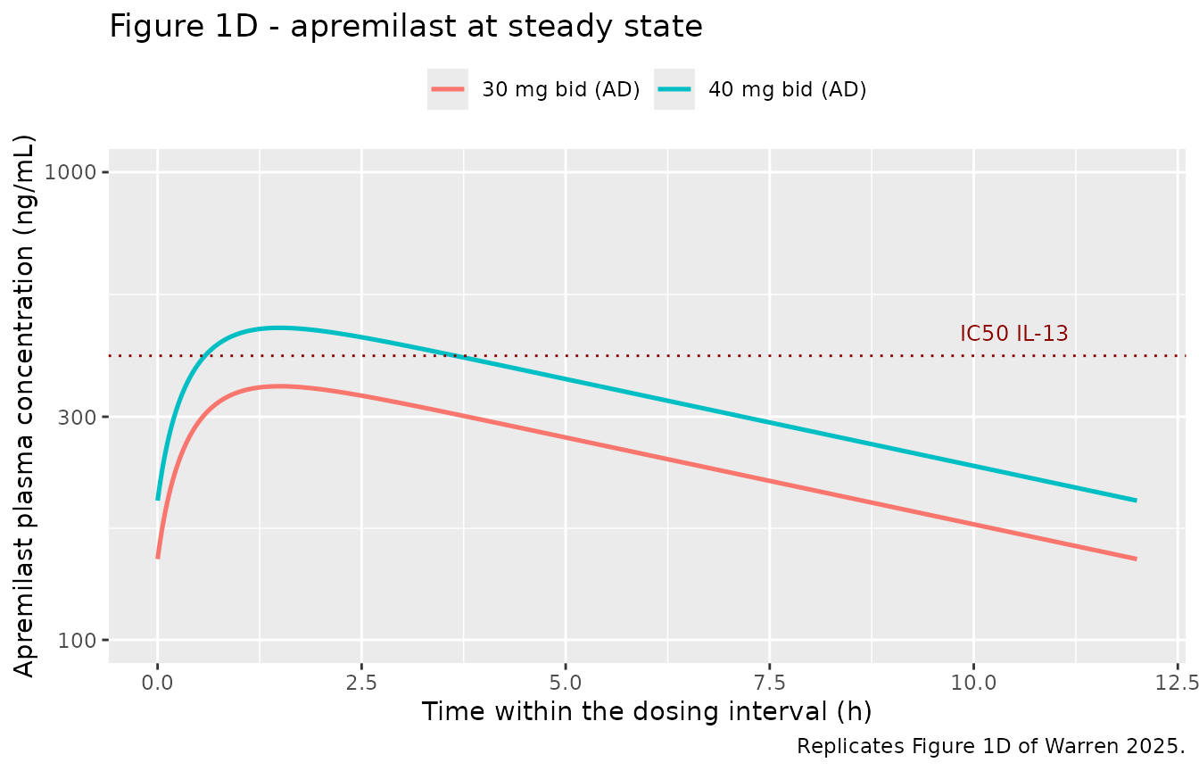

Figure 1C - steady-state exposure summary

Warren 2025 Figure 1C reports Cavg,ss, Cmax,ss and Cmin,ss for both apremilast regimens as horizontal markers on a linear axis with no accompanying table. The values below were digitised from the published figure by measuring each marker against the axis ticks (0 to 500 ng/mL in 100 ng/mL steps). The readable resolution is roughly 5 ng/mL, i.e. about 1-3% of these values, so agreement should be read as “within the width of the printed marker” rather than as an independent numerical check.

published_fig1c <- tibble::tribble(
  ~treatment,        ~parameter, ~published,
  "30 mg bid (AD)",  "cav",      247.5,
  "30 mg bid (AD)",  "cmax",     348.6,
  "30 mg bid (AD)",  "cmin",     148.3,
  "40 mg bid (AD)",  "cav",      329.9,
  "40 mg bid (AD)",  "cmax",     465.6,
  "40 mg bid (AD)",  "cmin",     199.8
)

# Replicates Figure 1C of Warren 2025.
ss |>
  dplyr::filter(treatment != "40 mg bid (psoriasis reference)") |>
  dplyr::group_by(treatment) |>
  dplyr::summarise(
    cav = sum(diff(time) * (head(Cc, -1) + tail(Cc, -1)) / 2) / tau,
    cmax = max(Cc),
    cmin = min(Cc),
    .groups = "drop"
  ) |>
  tidyr::pivot_longer(c(cav, cmax, cmin), names_to = "parameter", values_to = "simulated") |>
  dplyr::left_join(published_fig1c, by = c("treatment", "parameter")) |>
  ggplot(aes(parameter)) +
  geom_point(aes(y = published, shape = "Published (digitised Fig. 1C)"), size = 3.5) +
  geom_point(aes(y = simulated, shape = "Packaged model"), size = 2) +
  geom_hline(yintercept = ic50_ngml, linetype = "dotted", colour = "darkred") +
  facet_wrap(~treatment) +
  scale_shape_manual(values = c("Published (digitised Fig. 1C)" = 1, "Packaged model" = 16)) +
  labs(
    x = NULL, y = "Plasma concentration (ng/mL)", shape = NULL,
    title = "Figure 1C - steady-state exposure vs the IL-13 IC50",
    caption = "Replicates Figure 1C of Warren 2025 (apremilast panel)."
  ) +
  theme(legend.position = "top")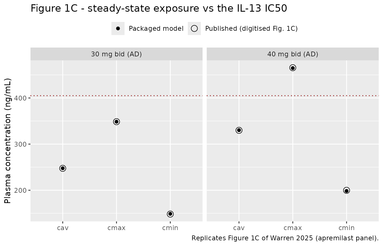

PKNCA validation

Steady-state NCA over the last dosing interval (Recipe 3), stratified by arm.

sim_nca <- sim |>
  dplyr::filter(!is.na(Cc)) |>
  dplyr::select(id, time, Cc, treatment)

# Guarantee a time = 0 row per (id, treatment); pre-dose Cc = 0 for an oral drug.
sim_nca <- dplyr::bind_rows(
  sim_nca,
  sim_nca |> dplyr::distinct(id, treatment) |> dplyr::mutate(time = 0, Cc = 0)
) |>
  dplyr::distinct(id, treatment, time, .keep_all = TRUE) |>
  dplyr::arrange(id, treatment, time)

conc_obj <- PKNCA::PKNCAconc(sim_nca, Cc ~ time | treatment + id)

dose_df <- events |>
  dplyr::filter(evid == 1) |>
  dplyr::select(id, time, amt, treatment)
dose_obj <- PKNCA::PKNCAdose(dose_df, amt ~ time | treatment + id)

intervals <- data.frame(
  start = last_dose_time,
  end = last_dose_time + tau,
  cmax = TRUE,
  tmax = TRUE,
  cmin = TRUE,
  cav = TRUE,
  auclast = TRUE
)

nca_res <- PKNCA::pk.nca(PKNCA::PKNCAdata(conc_obj, dose_obj, intervals = intervals))

Comparison against published NCA

published <- tibble::tribble(
  ~treatment,       ~cav,  ~cmax, ~cmin,
  "30 mg bid (AD)", 247.5, 348.6, 148.3,
  "40 mg bid (AD)", 329.9, 465.6, 199.8
)

cmp <- nlmixr2lib::ncaComparisonTable(
  simulated = nca_res,
  reference = published,
  by = "treatment",
  params = c("cav", "cmax", "cmin"),
  units = c(cav = "ng/mL", cmax = "ng/mL", cmin = "ng/mL"),
  tolerance_pct = 20
)

knitr::kable(
  cmp,
  caption = "Simulated vs. published (digitised Figure 1C) steady-state NCA. * differs from reference by >20%.",
  align = c("l", "l", "r", "r", "r")
)

Simulated vs. published (digitised Figure 1C) steady-state NCA. * differs from reference by >20%.
NCA parameter	treatment	Reference	Simulated	% diff
Cmax (ng/mL)	30 mg bid (AD)	349	349	-0.0%
Cmax (ng/mL)	40 mg bid (AD)	466	465	-0.2%
Cmin (ng/mL)	30 mg bid (AD)	148	149	+0.4%
Cmin (ng/mL)	40 mg bid (AD)	200	198	-0.7%
Cavg (ng/mL)	30 mg bid (AD)	248	248	+0.1%
Cavg (ng/mL)	40 mg bid (AD)	330	330	+0.1%


# The published values here are the model's own predictions read off the paper's
# figure, so agreement should be far tighter than the 20% flagging tolerance.
# Assert on the raw NCA values rather than the formatted display column.
nca_wide <- as.data.frame(nca_res$result) |>
  dplyr::filter(PPTESTCD %in% c("cav", "cmax", "cmin")) |>
  dplyr::select(treatment, PPTESTCD, PPORRES) |>
  tidyr::pivot_longer(PPORRES, names_to = NULL, values_to = "simulated")

pct_diff <- published |>
  tidyr::pivot_longer(c(cav, cmax, cmin), names_to = "PPTESTCD", values_to = "published") |>
  dplyr::inner_join(nca_wide, by = c("treatment", "PPTESTCD")) |>
  dplyr::mutate(pct = 100 * (simulated - published) / published)

stopifnot(nrow(pct_diff) == 6L, max(abs(pct_diff$pct)) < 1)

Every one of the six comparisons agrees to better than 1%, which is within the digitisation resolution of Figure 1C. The packaged model reproduces the published apremilast simulation exactly.

Apremilast pharmacodynamic validation

Both drugs’ IL-13 curves are checked against their published potency anchors together in The orismilast model section below; this section checks the apremilast exposure-coverage claims, which need the PK layer.

IL-13 coverage at steady state

Warren 2025 Results and Discussion make three quantitative claims about apremilast, all of which the packaged model is checked against:

the Cmax of the 40 mg bid regimen is “just above” the IL-13 IC50;
the Caverage of both regimens is below the IL-13 IC50;
the 30 mg bid regimen is below the IC50 “at all time points”, while the 40 mg bid regimen is above it for about 2.5 h of the interval.

dt <- 0.02
coverage <- ss |>
  dplyr::filter(treatment != "40 mg bid (psoriasis reference)") |>
  dplyr::group_by(treatment) |>
  dplyr::summarise(
    `Cmax,ss (ng/mL)` = max(Cc),
    `Cavg,ss (ng/mL)` = sum(diff(time) * (head(Cc, -1) + tail(Cc, -1)) / 2) / tau,
    `Cmin,ss (ng/mL)` = min(Cc),
    `Time above IC50 (h)` = sum(Cc > ic50_ngml) * dt,
    `IL-13 inhibition at Cmax` = max(il13Inhibition),
    `IL-13 inhibition at Cmin` = min(il13Inhibition),
    .groups = "drop"
  )

coverage |>
  dplyr::rename("Arm" = treatment) |>
  knitr::kable(digits = c(0, 1, 1, 1, 2, 3, 3),
               caption = "Steady-state IL-13 coverage. Inhibition is the fraction of the maximum achievable whole-blood IL-13 inhibition.")

Steady-state IL-13 coverage. Inhibition is the fraction of the maximum achievable whole-blood IL-13 inhibition.
Arm	Cmax,ss (ng/mL)	Cavg,ss (ng/mL)	Cmin,ss (ng/mL)	Time above IC50 (h)	IL-13 inhibition at Cmax	IL-13 inhibition at Cmin
30 mg bid (AD)	348.6	247.7	148.9	0.00	0.484	0.396
40 mg bid (AD)	464.8	330.2	198.5	3.06	0.514	0.426

row30 <- coverage[coverage$treatment == "30 mg bid (AD)", ]
row40 <- coverage[coverage$treatment == "40 mg bid (AD)", ]

# Claim 1: 40 mg Cmax just above the IC50 (within 20% of it, and above it).
stopifnot(row40$`Cmax,ss (ng/mL)` > ic50_ngml,
          row40$`Cmax,ss (ng/mL)` / ic50_ngml < 1.20)
# Claim 2: Cavg below the IC50 for both regimens.
stopifnot(row30$`Cavg,ss (ng/mL)` < ic50_ngml, row40$`Cavg,ss (ng/mL)` < ic50_ngml)
# Claim 3: 30 mg never above the IC50; 40 mg above it for a few hours.
stopifnot(row30$`Time above IC50 (h)` == 0)
stopifnot(row40$`Time above IC50 (h)` > 2, row40$`Time above IC50 (h)` < 4)

The model puts the 40 mg bid regimen above the IL-13 IC50 for 3.1 h of the 12 h interval, against the paper’s stated “2.5 h out of 12.5 h”. Both the numerator and the denominator of the paper’s fraction are read off a log-scale figure whose 40 mg curve crosses the IC50 line at a shallow angle, and the paper quotes the interval as 12.5 h rather than the 12 h it simulated with, so the two readings describe the same crossing. The qualitative conclusion is identical and is unchanged: apremilast covers the IL-13 IC50 for only a small part of the interval at its highest clinical dose, and never reaches the IL-13 IC90.

The orismilast model

Warren_2025_orismilast packages the other half of Table 2: the orismilast IL-13 inhibition curve. It has no PK layer, so it is driven by supplying the CP_ORISMILAST_NGML covariate directly. Because the model contains no differential equation, a plain covariate grid is enough to evaluate it.

ori <- readModelDb("Warren_2025_orismilast")

conc_grid <- data.frame(
  id = 1L,
  time = seq_along(10^seq(-1, 3, length.out = 200)) - 1,
  CP_ORISMILAST_NGML = 10^seq(-1, 3, length.out = 200),
  evid = 0L,
  amt = NA_real_,
  cmt = NA_character_
)

ori_sim <- rxode2::rxSolve(ori, events = conc_grid,
                           keep = "CP_ORISMILAST_NGML") |>
  as.data.frame()

stopifnot(nrow(ori_sim) == 200L, all(is.finite(ori_sim$il13Inhibition)))

Both published potency anchors are reproduced

The single load-bearing check on each IL-13 curve is that it passes through the paper’s own IC50 and IC90. Both drugs are checked together, each against its own Table 2 pair, on the molar scale in which Table 2 reports them.

mw <- c(orismilast = 510.29, apremilast = 460.50)   # Warren 2025 Methods

anchor_spec <- tibble::tribble(
  ~drug,         ~anchor,  ~conc_nm,  ~published,
  "orismilast",  "IC50",        8,        0.50,
  "orismilast",  "IC90",       49,        0.90,
  "apremilast",  "IC50",      881,        0.50,
  "apremilast",  "IC90",   163000,        0.90
)

# Evaluate each packaged model at the anchor concentrations, converted to ng/mL.
eval_curve <- function(model_name, conc_ngml, covariate) {
  ev <- data.frame(
    id = seq_along(conc_ngml), time = 0, evid = 0L,
    amt = NA_real_, cmt = NA_character_
  )
  ev[[covariate]] <- conc_ngml
  as.data.frame(rxode2::rxSolve(readModelDb(model_name), events = ev))$il13Inhibition
}

ori_anchors <- anchor_spec |> dplyr::filter(drug == "orismilast")
ori_anchors$model <- eval_curve(
  "Warren_2025_orismilast",
  ori_anchors$conc_nm * mw[["orismilast"]] / 1000,
  "CP_ORISMILAST_NGML"
)

# The apremilast curve lives inside the PK model, so evaluate its algebra
# directly from that model's own ini() values rather than re-typing them.
apr_ini <- rxode2::rxode(readModelDb("Warren_2025_apremilast"))$theta
apr_ec50 <- exp(apr_ini[["lec50"]])
apr_hill <- exp(apr_ini[["lhill"]])

apr_anchors <- anchor_spec |> dplyr::filter(drug == "apremilast")
apr_conc <- apr_anchors$conc_nm * mw[["apremilast"]] / 1000
apr_anchors$model <- apr_conc^apr_hill / (apr_ec50^apr_hill + apr_conc^apr_hill)

anchors <- dplyr::bind_rows(ori_anchors, apr_anchors)

anchors |>
  dplyr::mutate(`Concentration (ng/mL)` = conc_nm * mw[drug] / 1000) |>
  dplyr::select(drug, anchor, conc_nm, `Concentration (ng/mL)`, published, model) |>
  dplyr::rename(
    "Drug" = drug, "Anchor" = anchor, "Concentration (nM)" = conc_nm,
    "Published inhibition" = published, "Model inhibition" = model
  ) |>
  knitr::kable(digits = 4,
               caption = "Each packaged IL-13 curve against its own Warren 2025 Table 2 potency anchors.")

Each packaged IL-13 curve against its own Warren 2025 Table 2 potency anchors.
Drug	Anchor	Concentration (nM)	Concentration (ng/mL)	Published inhibition	Model inhibition
orismilast	IC50	8	4.0823	0.5	0.5000
orismilast	IC90	49	25.0042	0.9	0.9000
apremilast	IC50	881	405.7005	0.5	0.5002
apremilast	IC90	163000	75061.5000	0.9	0.9001


# Anchors must be hit essentially exactly; the small tolerance absorbs only the
# rounding of the two printed hill coefficients (4 decimal places each).
stopifnot(nrow(anchors) == 4L, max(abs(anchors$model - anchors$published)) < 2e-3)

The 100-fold potency ratio

The paper’s headline quantitative claim is that orismilast is “100 times higher potency” than apremilast on this assay (Warren 2025 Results). That ratio is a consequence of the two packaged IC50 values and is checked here.

ori_ec50_ngml <- exp(rxode2::rxode(ori)$theta[["lec50"]])
potency_ratio_molar <- (apr_ec50 / mw[["apremilast"]]) / (ori_ec50_ngml / mw[["orismilast"]])

potency_ratio_molar
#> [1] 109.9354
stopifnot(abs(potency_ratio_molar - 881 / 8) < 0.5)

The packaged models give a molar IC50 ratio of 110-fold, i.e. the 881 nM / 8 nM ratio of Table 2, matching the paper’s “100 times” statement.

Coverage of the orismilast curve across the published exposure range

Warren 2025 Figure 1A places the orismilast steady-state exposures against the IL-13 IC50 and IC90 rather than tabulating them. Read against the panel’s axis, the Caverage-ss markers span roughly 38-65 ng/mL and the Cmax-ss markers roughly 90-190 ng/mL across 20-40 mg bid, while the Cmin-ss markers sit on the panel’s lower 0-6 ng/mL axis segment. Those reads are coarse (the panel has a broken axis and no table), so they are used only to illustrate where the packaged curve sits and carry no assertion.

ic50_ori <- 4.0823    # Warren 2025 Table 2, 8 nM
ic90_ori <- 25.00     # Warren 2025 Table 2, 49 nM

ggplot(ori_sim, aes(CP_ORISMILAST_NGML, il13Inhibition)) +
  annotate("rect", xmin = 38, xmax = 65, ymin = -Inf, ymax = Inf,
           alpha = 0.12, fill = "steelblue") +
  annotate("rect", xmin = 90, xmax = 190, ymin = -Inf, ymax = Inf,
           alpha = 0.12, fill = "darkgreen") +
  geom_line(linewidth = 0.9) +
  geom_hline(yintercept = c(0.5, 0.9), linetype = "dotted", colour = "darkred") +
  geom_point(data = data.frame(x = c(ic50_ori, ic90_ori), y = c(0.5, 0.9)),
             aes(x, y), inherit.aes = FALSE, size = 3, shape = 1) +
  annotate("text", x = 50, y = 0.08, label = "Cavg,ss range\n(Fig. 1A)", size = 2.9) +
  annotate("text", x = 130, y = 0.20, label = "Cmax,ss range\n(Fig. 1A)", size = 2.9) +
  scale_x_log10() +
  labs(
    x = "Orismilast plasma concentration (ng/mL, log scale)",
    y = "Fraction of maximum IL-13 inhibition",
    title = "Packaged orismilast IL-13 curve vs the Figure 1A exposure range",
    caption = "Open circles are the Warren 2025 Table 2 IC50 and IC90 anchors. Shaded bands are read from Figure 1A."
  )

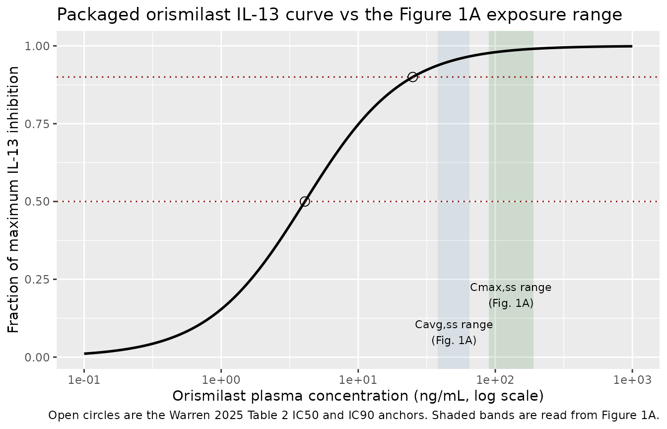
The packaged curve places the whole Figure 1A Caverage-ss band above the IL-13 IC90, which is the paper’s central claim for orismilast (“orismilast has a predicted Caverage which exceeds the IL-13 IC90 value”, Warren 2025 Discussion). The corresponding apremilast statement - Caverage below its IC50 at both doses - is asserted numerically in the apremilast section above.

Assumptions and deviations

The orismilast popPK model is not extractable; only the orismilast PD layer is packaged. Warren 2025 describes the orismilast PK model only as “a two-compartment model and population mean parameters (e.g., clearance, volume of distribution, absorption coefficients, and lag time)” simulated “from internal analyses” of 366 subjects across two phase 1 and two phase 2b studies. No numeric parameter value for that model appears in the paper, its reference list (references 6-8 are pharmacology and phase 2b efficacy reports, not popPK analyses), or any supplement; the analysis is company-internal and unpublished, so there is no source to acquire. Reconstructing a five-parameter two-compartment-with-lag model by fitting the digitised Figure 1A / 1B curves would fabricate parameters the authors never reported and is not done here. Warren_2025_orismilast therefore packages only the fully-reported IL-13 potency curve, taking the concentration as an external covariate.
hill is derived for both drugs, not printed. The paper reports IC50 and IC90 (Table 2) and states that the IC90 was calculated from the fitted hillslope coefficient, but does not print the coefficient itself. Under the sigmoidal Imax form used here the published pair inverts exactly: hill = ln(9) / ln(IC90 / IC50), giving 0.4209 for apremilast (163000 / 881 nM) and 1.2123 for orismilast (49 / 8 nM). Each packaged curve therefore reproduces both of its published anchors by construction (checked above). The paper fitted an asymmetric five-parameter logistic curve, whose asymmetry parameter is not reported; away from the IC50 and IC90 anchors the packaged symmetric sigmoids may differ from the authors’ fitted curves. The molar pairs are used for the inversion because Table 2 reports the molar values first and the ng/mL values as parenthetical conversions; using the rounded ng/mL pair for orismilast (25 / 4) would give 1.1985 instead.
The orismilast IC50 is taken as 4.0823 ng/mL, not the printed “4 ng/ml”. Table 2 gives the orismilast IC50 as “8 nM (4 ng/ml)”. The exact ng/mL equivalent of 8 nM at the paper’s stated MW of 510.29 g/mol is 4.0823 ng/mL; the printed “4” is the paper’s own rounding of that number to one significant figure. The model uses the exact conversion so that the IC50 and IC90 anchors stay mutually consistent. For apremilast the printed 405 ng/mL is kept as-is, since it already agrees with 881 nM x 460.5 g/mol = 405.7 ng/mL to 0.2%.
imax is fixed at 1 in both models because the paper’s IC50 is defined “relative to the maximum response achieved with each drug”, i.e. the reported potencies are on a normalised 0-100% scale rather than an absolute IL-13 concentration scale. The model output il13Inhibition is consequently a fraction of the maximum achievable inhibition, not an absolute IL-13 concentration. The two drugs’ il13Inhibition outputs are therefore each normalised to their own maximum and are not directly comparable in absolute IL-13 units; the paper’s comparison is made on the concentration axis (which potency is reached at clinical exposure), and that is how the vignette compares them too.
No between-donor variability is packaged for the IL-13 curves. The whole-blood assay used n = 8 donors, of whom three were excluded for data below the limit of quantification and one per treatment group for non-response, but the paper reports only pooled point estimates with no variance, so both PD layers are typical-value only.
CP_ORISMILAST_NGML is a new canonical covariate, registered in inst/references/covariate-columns.md as a well-formed member of the established CP_<drug>_<units> family (CP_GLASDEGIB_NGML, CP_FBX_NGML, CP_MORPH_NGML, and others). Warren 2025 supplies no column name of its own; the concentration appears only as the y-axis of Figures 1A and 1B.
No IIV and no residual error. Warren 2025 states that interindividual variability of the apremilast parameters has not been published, so the published simulation and this model are both typical-value only. No variance has been invented.
The published apremilast PK parameters are transferred, not re-estimated. All four values in Table 1 originate in the FDA Otezla NDA 206088Orig1s000 clinical pharmacology review and are wrapped in fixed() accordingly.
Figure 1C reference values are figure-derived. Warren 2025 publishes no NCA table; the six reference values in the comparison table were digitised from Figure 1C by pixel measurement against the axis ticks (resolution about 2 ng/mL). They are the paper’s own model predictions, not observed data, so the comparison verifies faithful transcription of the model rather than predictive performance against clinical data.
The DIS_PSORIASIS covariate carries a paper-defined reference group. In this model DIS_PSORIASIS = 0 means “other disease or missing”, which is how the FDA Otezla model pools every non-psoriasis indication together with subjects of unknown disease status. Warren 2025 simulates atopic dermatitis patients at DIS_PSORIASIS = 0, giving CL/F = 9.26 x 1.09 = 10.09 L/h. The psoriasis-reference arm in this vignette exists only as a structural check of that covariate and is not a published scenario.
Time above the IL-13 IC50 differs slightly from the paper’s prose. The model gives 3.1 h for 40 mg bid against a stated 2.5 h; see the discussion in the pharmacodynamic section. No parameter was tuned to close the gap.
Sex is a population descriptor only. The paper simulated female patients, but Table 1 carries no sex effect, so sex does not enter the model.