Ceftolozane/tazobactam and imipenem resistance in P. aeruginosa ampC/ampD mutants (Deroche 2023)
Source:vignettes/articles/Deroche_2023_ceftolozane_imipenem_resistance.Rmd
Deroche_2023_ceftolozane_imipenem_resistance.RmdModel and source
- Citation: Deroche L, Plouzeau C, Bemer P, Dalichampt M, Michaud A, Chavanet P, Burucoa C, Rammaert B, Gregoire N, Marchand S, Cremniter J. Characterization of Pseudomonas aeruginosa resistance to ceftolozane-tazobactam due to ampC and/or ampD mutations observed during treatment using semi-mechanistic PKPD modeling. Antimicrob Agents Chemother. 2023 Oct 18;67(10):e00480-23. doi:10.1128/aac.00480-23. PMID:37695298; PMCID:PMC10583683. Structural model: effect Eq 1 (main text), adaptation Eqs 2-3 (main text), full differential equations Suppl Text S1 Eqs 2-6, schematic Fig 5. Parameter estimates: Table S2.
- Article: https://doi.org/10.1128/aac.00480-23
This is not a population PK model. It is a semi-mechanistic time-kill PK/PD model with adaptation (the Mouton model, Deroche 2023 Discussion and refs 15, 27, 28) fit in NONMEM 7.4 (Laplacian, Beal M3 for below-quantification data) to bacterial-count data (log10 CFU/mL) from sequential in-vitro time-kill curves (TKCs) against Pseudomonas aeruginosa. The paper studies how two chromosomal mutations observed in a patient treated with ceftolozane/tazobactam (C/T) – AmpC G183D and AmpD H157Y – change susceptibility to C/T and to imipenem (IMI).
Because there is no absorption-distribution-elimination PK profile to integrate, PKNCA is not an appropriate validation. The checks below are the mechanistic equivalents: the structural identities of the adaptation model, exact reproduction of the paper’s EC50,off->on-versus-time simulations (Figs 2 and 4), and qualitative reproduction of the killing / regrowth time-kill curves (Figs 1 and 3).
The 11 packaged models
The paper fits the same structural model independently to each
strain, with the maximum effect emax and the adaptation
rate kon shared within a strain group. nlmixr2lib therefore
ships one model file per strain-by-drug combination (11 in total), all
pointing to this vignette:
ct_strains  <- c("PAO1", "AmpC", "AmpD", "AmpCD", "PaS", "PaR", "PaRrev")
imi_strains <- c("PAO1", "AmpC", "AmpD", "AmpCD")
ct_models  <- paste0("Deroche_2023_ceftolozanetazobactam_", ct_strains)
imi_models <- paste0("Deroche_2023_imipenem_", imi_strains)
all_models <- c(ct_models, imi_models)
data.frame(
  drug = c(rep("C/T", length(ct_models)), rep("IMI", length(imi_models))),
  model = all_models
) |>
knitr::kable(caption = "The 11 strain-by-drug model files from Deroche 2023.")| drug | model |
|---|---|
| C/T | Deroche_2023_ceftolozanetazobactam_PAO1 |
| C/T | Deroche_2023_ceftolozanetazobactam_AmpC |
| C/T | Deroche_2023_ceftolozanetazobactam_AmpD |
| C/T | Deroche_2023_ceftolozanetazobactam_AmpCD |
| C/T | Deroche_2023_ceftolozanetazobactam_PaS |
| C/T | Deroche_2023_ceftolozanetazobactam_PaR |
| C/T | Deroche_2023_ceftolozanetazobactam_PaRrev |
| IMI | Deroche_2023_imipenem_PAO1 |
| IMI | Deroche_2023_imipenem_AmpC |
| IMI | Deroche_2023_imipenem_AmpD |
| IMI | Deroche_2023_imipenem_AmpCD |
Population (biological context)
The structural data come from a single patient case: a 58-year-old woman on breast-cancer chemotherapy developed a catheter-related P. aeruginosa bacteremia. A C/T-susceptible isolate (PaS, C/T MIC 1 mg/L) was recovered before treatment and a C/T-resistant isolate (PaR, C/T MIC 32 mg/L) after two weeks of C/T. Whole-genome sequencing showed the two isolates were isogenic (ST252) and differed in, among others, the AmpC G183D and AmpD H157Y substitutions. To isolate the effect of each mutation, the authors recreated them in the reference strain PAO1 by scarless homologous recombination (PAO1-AmpCG183D, PAO1-AmpDH157Y, PAO1-AmpCG183D/AmpDH157Y) and reverted them in PaR (PaR-AmpCPaS/AmpDPaS).
All time-kill experiments were run in cation-adjusted Mueller-Hinton broth II at 35 C, inoculated at 1e6 CFU/mL, with sampling at 0, 3, 6, 24 and 30 h and a 200 CFU/mL limit of quantification. A second TKC was started at 24 h from the regrowth wells of the first, at antibiotic concentrations up to 64x MIC. To offset imipenem degradation (half-life 16.4 h) the IMI wells were re-dosed at 9 and 24 h (44% and 35% of the initial dose).
The same context is available programmatically via
readModelDb("Deroche_2023_ceftolozanetazobactam_PaR")$population.
Structural model
Per-parameter origins are recorded as in-file comments next to each
ini() entry in each model file. All numeric values are the
final estimates from Deroche 2023 Tables S2 (PAO1 C/T), S3 (clinical
C/T) and S4 (PAO1 IMI), with 95% confidence intervals determined by
sampling-importance-resampling.
The system has three states (Deroche 2023 Fig 5; Suppl Text S1 Eqs 2-6):
-
bacteria– viable count (CFU/mL), dosed as the inoculum, -
aroff– fraction of non-adapted bacteria, starting at 1, -
aron– fraction of adapted bacteria, starting at 0,
plus cdrug, the user-dosed static drug
concentration.
| Equation | Form | Source |
|---|---|---|
| Growth | d/dt(bacteria) = knet*(1 - bacteria/Bmax)*Delay*bacteria - Effect*bacteria |
Suppl Eq 2 |
| Non-adapted fraction | d/dt(aroff) = koff*aron - kon*aroff |
Suppl Eq 3 |
| Adapted fraction | d/dt(aron) = kon*aroff - koff*aron |
Suppl Eq 4 |
| Drug effect | Effect = Emax*C/(EC50off + C)*aroff + Emax*C/(EC50on + C)*aron |
Eq 1 / Suppl Eq 5 |
| Growth lag | Delay = Time^20/(Tlag^20 + Time^20) |
Suppl Eq 6 |
Because koff is fixed to 0, the adaptation equations
have the closed-form solution aroff(t) = exp(-kon*t),
aron(t) = 1 - exp(-kon*t) (Eqs 2-3 of the main text). Two
drugs, three strain groups, and the shared emax /
kon per group:
grp <- function(m) {
  p <- rxode2::rxode(readModelDb(m))$theta
  c(emax = unname(p[["emax"]]), kon = unname(p[["kon"]]))
}
data.frame(
  group = c("PAO1 (C/T)", "clinical (C/T)", "PAO1 (IMI)"),
  rbind(grp("Deroche_2023_ceftolozanetazobactam_PAO1"),
        grp("Deroche_2023_ceftolozanetazobactam_PaS"),
        grp("Deroche_2023_imipenem_PAO1"))
) |>
  knitr::kable(digits = 4,
caption = "Emax (1/h) and kon (1/h) shared within each strain group (Tables S2-S4).")| group | emax | kon |
|---|---|---|
| PAO1 (C/T) | 1.94 | 0.0897 |
| clinical (C/T) | 3.09 | 0.0614 |
| PAO1 (IMI) | 4.71 | 0.0640 |
Strain-specific parameter table (file vs. paper)
grab <- function(m) {
  p <- rxode2::rxode(readModelDb(m))$theta
  data.frame(
    model = m,
    knet = unname(p[["knet"]]),
    log10bmax = unname(p[["log10bmax"]]),
    ec50off = unname(p[["ec50off"]]),
    ec50on = unname(p[["ec50on"]])
  )
}
do.call(rbind, lapply(all_models, grab)) |>
  knitr::kable(
    digits = 4,
    row.names = FALSE,
    caption = "Strain-specific estimates as loaded from the model files (Deroche 2023 Tables S2-S4)."
)| model | knet | log10bmax | ec50off | ec50on |
|---|---|---|---|---|
| Deroche_2023_ceftolozanetazobactam_PAO1 | 1.380 | 10.00 | 0.0444 | 0.551 |
| Deroche_2023_ceftolozanetazobactam_AmpC | 0.823 | 9.97 | 0.0606 | 19.400 |
| Deroche_2023_ceftolozanetazobactam_AmpD | 0.873 | 9.98 | 0.1810 | 2.200 |
| Deroche_2023_ceftolozanetazobactam_AmpCD | 0.824 | 10.00 | 1.2900 | 70.800 |
| Deroche_2023_ceftolozanetazobactam_PaS | 0.891 | 9.44 | 1.3600 | 155.000 |
| Deroche_2023_ceftolozanetazobactam_PaR | 0.901 | 9.38 | 80.5000 | 420.000 |
| Deroche_2023_ceftolozanetazobactam_PaRrev | 0.768 | 9.07 | 6.7700 | 269.000 |
| Deroche_2023_imipenem_PAO1 | 2.120 | 9.93 | 0.4110 | 24.800 |
| Deroche_2023_imipenem_AmpC | 0.684 | 9.95 | 1.8600 | 2.250 |
| Deroche_2023_imipenem_AmpD | 1.870 | 9.63 | 2.0300 | 7.680 |
| Deroche_2023_imipenem_AmpCD | 1.110 | 9.86 | 0.4940 | 3.290 |
Check 1 – EC50,off and EC50,on anchor the effect model exactly
The two per-strain potencies are the drug concentrations giving 50%
of Emax when 0% (EC50off) and 100%
(EC50on) of the bacteria are adapted. They should therefore
be recoverable as the roots of Effect(C) = 0.5*Emax
evaluated with aron = 0 and aron = 1. This is
an exact structural identity: it confirms the effect equation and the
loaded potencies agree with Tables 1 and 2.
# EC50 of a single Emax term: Effect = Emax*C/(EC50 + C); at C = EC50, Effect = Emax/2.
# For the mixed effect at adapted fraction f:
ec50_at <- function(emax, eoff, eon, f) {
  uniroot(function(C) (1 - f) * C / (eoff + C) + f * C / (eon + C) - 0.5,
          c(1e-10, 1e8), tol = 1e-12)$root
}
anchor <- do.call(rbind, lapply(all_models, function(m) {
  p <- rxode2::rxode(readModelDb(m))$theta
  data.frame(
    model = m,
    ec50off_file = unname(p[["ec50off"]]),
    ec50_f0 = ec50_at(p[["emax"]], p[["ec50off"]], p[["ec50on"]], 0),
    ec50on_file = unname(p[["ec50on"]]),
    ec50_f1 = ec50_at(p[["emax"]], p[["ec50off"]], p[["ec50on"]], 1)
  )
}))
stopifnot(
  max(abs(anchor$ec50_f0 - anchor$ec50off_file)) < 1e-6,
  max(abs(anchor$ec50_f1 - anchor$ec50on_file)) < 1e-6
)
knitr::kable(anchor, digits = 4,
caption = "At 0% adapted the mixed EC50 equals EC50,off; at 100% adapted it equals EC50,on. Exact.")| model | ec50off_file | ec50_f0 | ec50on_file | ec50_f1 |
|---|---|---|---|---|
| Deroche_2023_ceftolozanetazobactam_PAO1 | 0.0444 | 0.0444 | 0.551 | 0.551 |
| Deroche_2023_ceftolozanetazobactam_AmpC | 0.0606 | 0.0606 | 19.400 | 19.400 |
| Deroche_2023_ceftolozanetazobactam_AmpD | 0.1810 | 0.1810 | 2.200 | 2.200 |
| Deroche_2023_ceftolozanetazobactam_AmpCD | 1.2900 | 1.2900 | 70.800 | 70.800 |
| Deroche_2023_ceftolozanetazobactam_PaS | 1.3600 | 1.3600 | 155.000 | 155.000 |
| Deroche_2023_ceftolozanetazobactam_PaR | 80.5000 | 80.5000 | 420.000 | 420.000 |
| Deroche_2023_ceftolozanetazobactam_PaRrev | 6.7700 | 6.7700 | 269.000 | 269.000 |
| Deroche_2023_imipenem_PAO1 | 0.4110 | 0.4110 | 24.800 | 24.800 |
| Deroche_2023_imipenem_AmpC | 1.8600 | 1.8600 | 2.250 | 2.250 |
| Deroche_2023_imipenem_AmpD | 2.0300 | 2.0300 | 7.680 | 7.680 |
| Deroche_2023_imipenem_AmpCD | 0.4940 | 0.4940 | 3.290 | 3.290 |
Check 2 – EC50,off->on over time reproduces Figs 2 and 4
The paper’s headline simulation is the empirical half-maximal
concentration EC50,off->on(t): the concentration at
which Effect = 0.5*Emax at time t, given the
adapted fraction aron(t) = 1 - exp(-kon*t). It rises from
EC50off at t = 0 to EC50on as the
population adapts. Time is measured from the start of the first TKC and
the simulations run to 54 h (Deroche 2023 Figs 2, 4).
ec50_time <- function(m, times) {
  p <- rxode2::rxode(readModelDb(m))$theta
  vapply(times, function(t) {
    f <- 1 - exp(-p[["kon"]] * t)
    ec50_at(p[["emax"]], p[["ec50off"]], p[["ec50on"]], f)
  }, numeric(1))
}
tt <- seq(0, 54, by = 0.5)
ct_curve <- do.call(rbind, lapply(ct_models[1:4], function(m)
  data.frame(strain = sub(".*_", "", m), time = tt, ec50 = ec50_time(m, tt))))
imi_curve <- do.call(rbind, lapply(imi_models, function(m)
  data.frame(strain = sub(".*_", "", m), time = tt, ec50 = ec50_time(m, tt))))
lab <- c(PAO1 = "PAO1", AmpC = "PAO1-AmpC(G183D)", AmpD = "PAO1-AmpD(H157Y)",
         AmpCD = "PAO1-AmpC/AmpD")
ct_curve$strain <- factor(lab[ct_curve$strain], levels = lab)
imi_curve$strain <- factor(lab[imi_curve$strain], levels = lab)
ggplot(ct_curve, aes(time, ec50, colour = strain)) +
  geom_line(linewidth = 1) +
  geom_vline(xintercept = 24, linetype = 2) +
  scale_y_log10() +
  labs(x = "Time (h)", y = expression(EC[50][", off->on"]~"(mg/L)"),
       colour = "Strain", title = "C/T adaptive resistance (Fig 2)")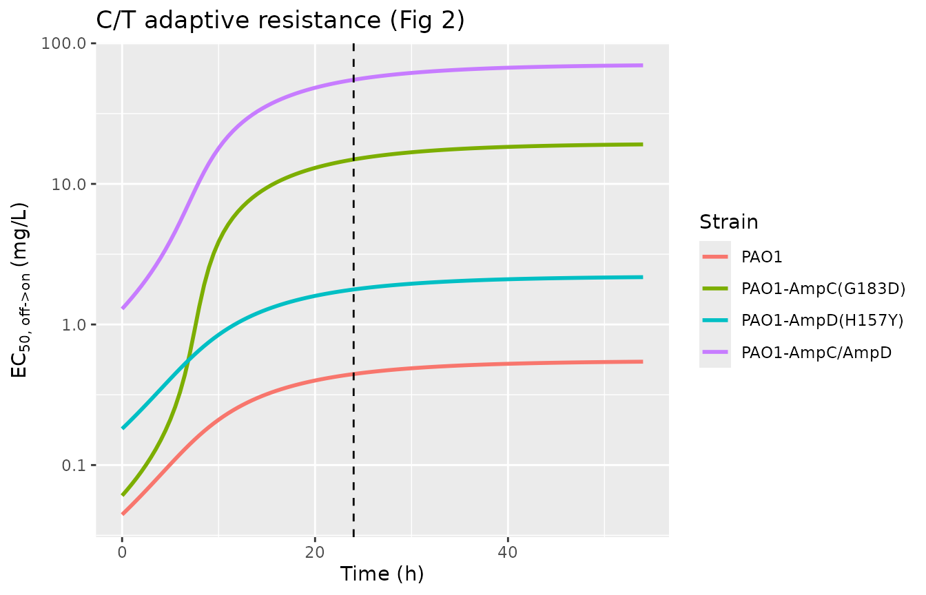
Replicates Figure 2 of Deroche 2023: EC50,off->on over time for C/T, PAO1 and mutant-derived strains.
ggplot(imi_curve, aes(time, ec50, colour = strain)) +
  geom_line(linewidth = 1) +
  geom_vline(xintercept = 24, linetype = 2) +
  scale_y_log10() +
  labs(x = "Time (h)", y = expression(EC[50][", off->on"]~"(mg/L)"),
       colour = "Strain", title = "Imipenem adaptive resistance (Fig 4)")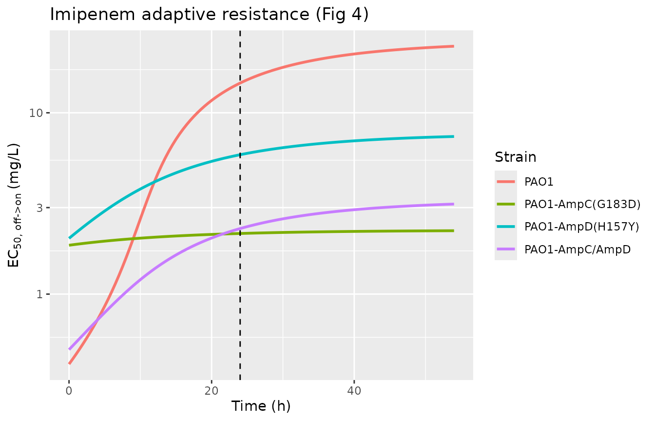
Replicates Figure 4 of Deroche 2023: EC50,off->on over time for imipenem, PAO1 and mutant-derived strains.
The endpoints of these curves are the Table 1 / Table 2 values: at
t = 0 the curve is at EC50off, and as the
population fully adapts it approaches EC50on. The paper
also states that “about 90% of adaptation [is] reached after 24 hours”
for the PAO1 C/T group; the shared kon reproduces this.
kon_ct <- rxode2::rxode(readModelDb("Deroche_2023_ceftolozanetazobactam_PAO1"))$theta[["kon"]]
adapt24 <- 1 - exp(-kon_ct * 24)
cat(sprintf("Adapted fraction at 24 h (C/T PAO1 group, kon = %.4f /h): %.1f%%\n",
            kon_ct, 100 * adapt24))
#> Adapted fraction at 24 h (C/T PAO1 group, kon = 0.0897 /h): 88.4%
stopifnot(abs(adapt24 - 0.90) < 0.05)
Check 3 – sequential kill curves reproduce Figs 1 and 3
A full simulation integrates all three states. The inoculum is dosed
to bacteria at the start of each TKC (an
evid = 5 replacement event reinoculates at 24 h), the drug
concentration is dosed to cdrug, and the occasion column
OCC selects the TKC-specific growth lag. The adapted
fraction develops continuously across both TKCs (it is not reset), so
the second TKC starts from an already-adapted population – the mechanism
that drives the regrowth seen at higher concentrations in the second
kill (Deroche 2023 Fig 1).
solve_tkc <- function(m, c1, c2) {
  mod <- rxode2::rxode(readModelDb(m))
  dose <- data.frame(
    id = 1L, time = c(0, 0, 24, 24), evid = c(1L, 1L, 5L, 5L),
    amt = c(1e6, c1, 1e6, c2), cmt = c("bacteria", "cdrug", "bacteria", "cdrug")
  )
  obs <- data.frame(
    id = 1L, time = sort(unique(c(seq(0, 24, 0.25), seq(24, 54, 0.25)))),
    evid = 0L, amt = NA_real_, cmt = "bacteria"
  )
  d <- rbind(dose, obs)
  d <- d[order(d$time, -d$evid), ]
  d$OCC <- ifelse(d$time < 24, 1L, 2L)
  # rxSolve returns observation rows only (no evid column).
  out <- rxode2::rxSolve(mod, d, returnType = "data.frame")
  out[, c("time", "log_cfu")]
}
For PAO1 against C/T (Fig 1A), the first TKC at concentrations around and above the MIC (0.25 mg/L) kills and regrows; the plot below shows the control (no drug), the MIC, and two higher concentrations across both sequential TKCs.
concs <- data.frame(label = c("control", "0.25 (MIC)", "1 mg/L", "4 mg/L"),
                    c1 = c(0, 0.25, 1, 4), c2 = c(0, 1, 4, 16))
ct1a <- do.call(rbind, Map(function(l, a, b) {
  s <- solve_tkc("Deroche_2023_ceftolozanetazobactam_PAO1", a, b)
  s$arm <- l; s
}, concs$label, concs$c1, concs$c2))
ct1a$arm <- factor(ct1a$arm, levels = concs$label)
ggplot(ct1a, aes(time, log_cfu, colour = arm)) +
  geom_line(linewidth = 0.9) +
  geom_vline(xintercept = 24, linetype = 2) +
  geom_hline(yintercept = log10(200), linetype = 3, colour = "grey50") +
  labs(x = "Time (h)", y = expression(log[10]~CFU/mL),
       colour = "C/T (TKC1 -> TKC2)", title = "C/T vs PAO1 (Fig 1A)",
       caption = "Dashed: second-TKC start. Dotted: 200 CFU/mL limit of quantification.")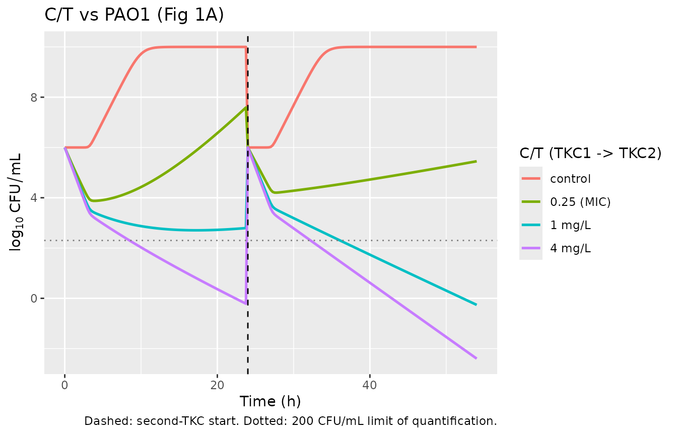
Representative C/T kill curves for PAO1 across the two sequential TKCs (compare Fig 1A). Second TKC uses fourfold-higher concentrations.
For PAO1 against imipenem (Fig 3A), the same qualitative pattern holds, with killing at concentrations above the IMI MIC of 0.5 mg/L.
concs_i <- data.frame(label = c("control", "0.5 (MIC)", "2 mg/L", "8 mg/L"),
                      c1 = c(0, 0.5, 2, 8), c2 = c(0, 2, 8, 32))
imi3a <- do.call(rbind, Map(function(l, a, b) {
  s <- solve_tkc("Deroche_2023_imipenem_PAO1", a, b)
  s$arm <- l; s
}, concs_i$label, concs_i$c1, concs_i$c2))
imi3a$arm <- factor(imi3a$arm, levels = concs_i$label)
ggplot(imi3a, aes(time, log_cfu, colour = arm)) +
  geom_line(linewidth = 0.9) +
  geom_vline(xintercept = 24, linetype = 2) +
  geom_hline(yintercept = log10(200), linetype = 3, colour = "grey50") +
  labs(x = "Time (h)", y = expression(log[10]~CFU/mL),
       colour = "IMI (TKC1 -> TKC2)", title = "Imipenem vs PAO1 (Fig 3A)",
       caption = "Dashed: second-TKC start. Dotted: 200 CFU/mL limit of quantification.")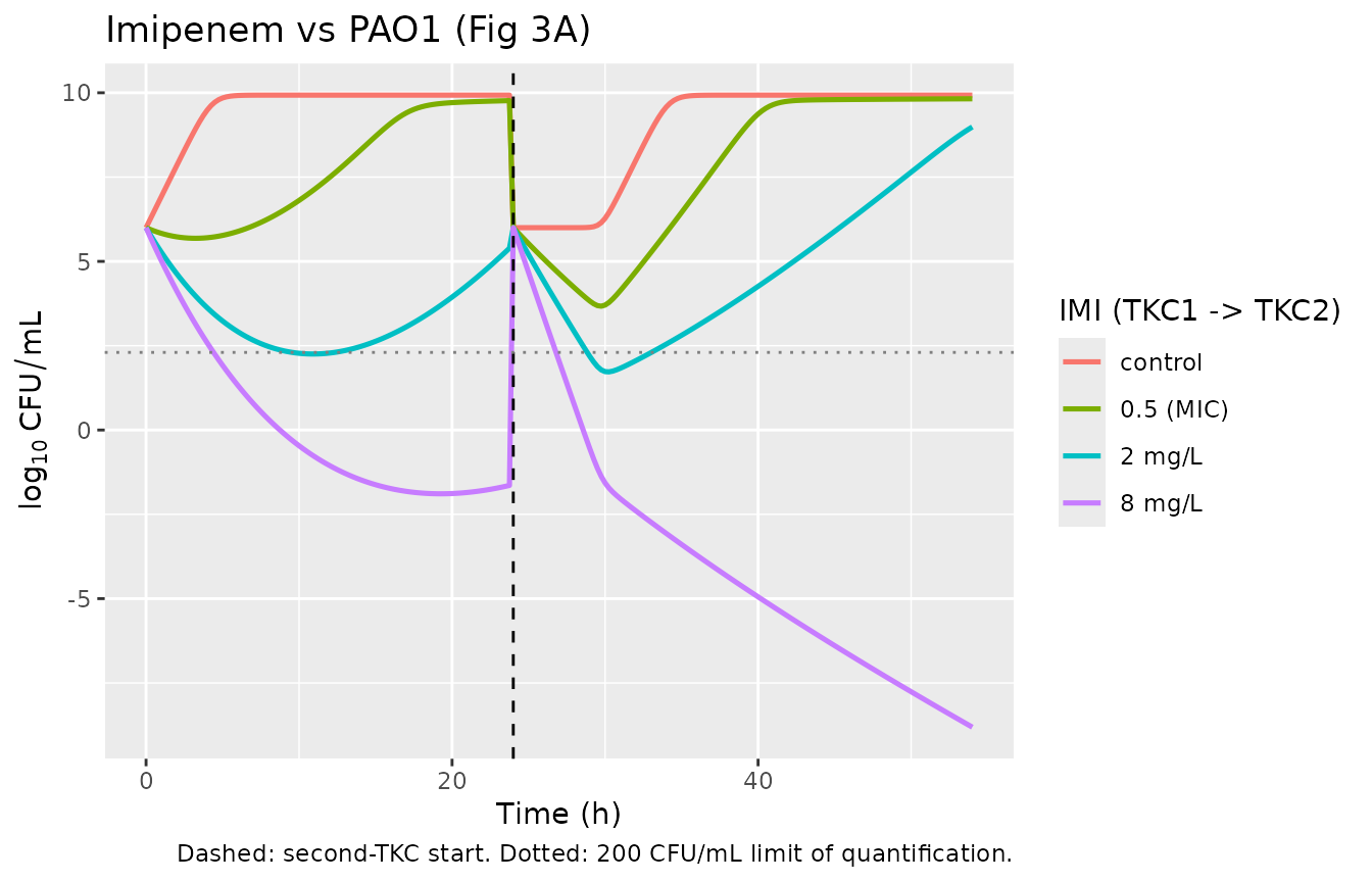
Representative imipenem kill curves for PAO1 across the two sequential TKCs (compare Fig 3A).
Check 4 – control growth reaches Bmax with the fitted lag
With no drug, the population grows from the inoculum to the strain’s
Bmax after the growth lag Tlag1. For PAO1
against C/T, Bmax = 10^10 CFU/mL and
Tlag1 = 3.24 h.
gc <- solve_tkc("Deroche_2023_ceftolozanetazobactam_PAO1", 0, 0)
# Restrict to the first TKC, before the 24-h reinoculation resets the count.
gc1 <- gc[gc$time < 24, ]
plateau <- tail(gc1$log_cfu, 1)
cat(sprintf("Inoculum log10 CFU/mL at t=0.25     : %.2f\n", gc1$log_cfu[1]))
#> Inoculum log10 CFU/mL at t=0.25     : 6.00
cat(sprintf("Plateau  log10 CFU/mL at t=23.75    : %.2f  (Bmax = 10 log10 CFU/mL)\n",
            plateau))
#> Plateau  log10 CFU/mL at t=23.75    : 10.00  (Bmax = 10 log10 CFU/mL)
stopifnot(abs(plateau - 10) < 0.2)
Assumptions and deviations
-
Drug concentration as a user-dosed state. The
time-kill experiments are static-concentration (the drug is held
constant within a TKC), so the drug is reproduced here as a single
concentration state
cdrug(mg/L) dosed by the user, following the convention of the other in-vitro time-kill models in the library. The experimental re-dosing of imipenem at 9 and 24 h to offset its degradation was a technique to maintain the nominal concentration; the PD model uses that nominal concentration directly (there is no drug-PK ODE in the published model), so it is not reproduced as a separate elimination term. -
Inoculum as a dose. The initial inoculum (1e6
CFU/mL, Methods) is applied as a dose to
bacteriarather than as an initial condition, so thattad(bacteria)provides the per-TKC growth-lag clock and the second-TKC reinoculation (evid = 5) resets it. The published model specifiesIC = 10^Inocwith a fixed inoculum; the value is identical, only the mechanism of setting it differs. -
Growth-lag reformulation. The published lag
function
Delay = Time^20/(Tlag^20 + Time^20)(Suppl Eq 6) is written in the algebraically identical reciprocal form1/(1 + (Tlag/Time)^20)so that a strain with a fixedTlag = 0givesDelay = 1att = 0without a 0/0 singularity. A negligible 1e-10 is added to the denominator time to avoid a division by zero exactly at an inoculation event. -
konunits. Table S2-S4 listkonwith units “h^-1 mg^-1 L”, but the supplement’s own adaptation equations (Suppl Eqs 3-4) and the main-text closed formARoff = exp(-kon*t)(Eq 2) usekonas a first-order rate in1/h, independent of concentration. The equation form is followed here (it reproduces Figs 2 and 4), per the standing rule to trust the equation over a conflicting table annotation. - Main-text vs supplement tables. Parameter values are taken from the supplement parameter tables (S2-S4). They agree with main-text Tables 1-2 except for rounding of the imipenem double-mutant EC50,off (Table 2: 0.495 mg/L; Table S4: 0.494 mg/L; the Table S4 value is used) and a misprinted upper confidence limit for the PaS EC50,on in Table 1 (“124-92”; Table S3 gives 124-192). Neither affects a point estimate used here.
-
No inter-strain random effects. The model is
deterministic: strain differences are captured by separate parameter
sets (one file each), not by random effects. The only stochastic element
in the paper is the additive residual error on log10 CFU/mL (variance
sigma^2, per strain), carried as
addSd = sqrt(sigma^2)for use in stochastic simulation. - Clinical isolates PaS/PaR. For the clinical pair the two resistance types (acquired, from mutations, and adaptive) cannot be separated, and the PaR isolate had already been exposed to C/T in vivo; the paper flags its first-TKC EC50,off as possibly already adapted. The estimates are shipped as reported (Table S3) for completeness.