Lumefantrine (Juma 2026)
Source:vignettes/articles/Juma_2026_lumefantrine.Rmd
Juma_2026_lumefantrine.RmdModel and source
mod_fn <- readModelDb("Juma_2026_lumefantrine")
mod    <- rxode2::rxode2(mod_fn())
#> Warning: some etas defaulted to non-mu referenced, possible parsing error: etaiov_ka_1, etaiov_ka_2, etaiov_fdepot_1, etaiov_fdepot_2
#> as a work-around try putting the mu-referenced expression on a simple line- Citation: Juma E, Ding J, Ongas M, Koskei N, Onyango K, Oloo F, Aman R, Kokwaro G, Tarning J, Ogutu B (2026). Population pharmacokinetics of lumefantrine in pregnant and non-pregnant women with uncomplicated Plasmodium falciparum malaria in Western Kenya. British Journal of Clinical Pharmacology 92(3):911-921. doi:10.1111/bcp.70318.
- Description: Population PK model for oral lumefantrine in 50 pregnant (second and third trimester) and 25 non-pregnant Kenyan women with uncomplicated Plasmodium falciparum malaria treated with the standard six-dose artemether-lumefantrine regimen (Juma 2026 Br J Clin Pharmacol). Absorption is a three-transit chain (ktr = 3 / MTT) feeding a separately estimated first-order absorption step (ka) into a two-compartment disposition model with first-order elimination. Relative bioavailability F is fixed at 1 for the population and carries a Box-Cox transformed inter-occasion random effect (lambda = -0.690) plus an a priori dose-saturable absorption term with Dose50 = 3.84 mg/kg. Allometric body weight scaling on all clearance (exponent 0.75) and volume (exponent 1) parameters centred at 70 kg. Pregnancy is a proportional covariate that increases CL/F by 23.2% and Vc/F by 28.1%, giving roughly 30% lower lumefantrine exposure in pregnant women. Inter-individual variability on MTT (CV 74.4%) and Vc/F (CV 14.1%); inter-occasion variability across two pooled dose occasions on ka (CV 109%) and F (CV 64.0%). Combined proportional (33.0%) and additive (12.0 ng/mL) residual error.
- Article: https://doi.org/10.1111/bcp.70318
Juma and colleagues studied lumefantrine after the standard six-dose artemether-lumefantrine regimen in pregnant and non-pregnant Kenyan women with uncomplicated Plasmodium falciparum malaria, and found that pregnancy raises apparent clearance by 23.2% and apparent central volume by 28.1%, lowering lumefantrine exposure by roughly 30%.
Population
Fifty pregnant women (30 in the second and 20 in the third trimester, gestational age median 26 weeks, range 13-40) and 25 non-pregnant women were enrolled at Ahero County Hospital in Kisumu County, western Kenya, between August 2013 and April 2014 (Pan African Clinical Trial Registry PACTR201211000451437). All participants were women aged 18-40 years with uncomplicated P. falciparum mono-infection (1000-200 000 parasites/uL), haemoglobin at least 8 g/dL, and no antimalarial exposure in the preceding month.
Baseline characteristics are in Table 1 of the source: median age 20.2 years (18.0-35.3) in pregnant and 25.2 years (18.1-35.6) in non-pregnant women; median body weight 62.0 kg (40.0-86.6) and 59.5 kg (45.0-89.0) respectively; median enrolment parasitaemia 10 960/uL and 24 320/uL. Every participant received four tablets of artemether/lumefantrine 20/120 mg (Coartem, Novartis AG), i.e. 480 mg lumefantrine per dose, at 0, 8, 24, 36, 48 and 60 h, taken with 250 mL of milk or a light meal. The day-28 PCR-corrected cure rate was 100% in both groups.
The population PK model was built in NONMEM 7.4 (FOCE-I) from 1151 venous plasma lumefantrine concentrations; 86 samples (7.4%) were below the 10 ng/mL LLOQ and were omitted (M1). Parameter uncertainty came from sampling importance resampling.
The same information is available programmatically via the model’s
population metadata
(readModelDb("Juma_2026_lumefantrine")()$population).
Source trace
Every ini() entry in
inst/modeldb/specificDrugs/Juma_2026_lumefantrine.R carries
an in-file comment naming its source location. They are collected here
for review.
| Equation / parameter | Value as encoded | Source location |
|---|---|---|
lmtt |
log(4.70) h |
Table 2, MTT (h) = 4.70 (RSE 6.9%) |
| transit chain length | 3 transit compartments | Table 2, No. transit comp. = 3 (fixed); Figure 1 |
lka |
log(0.411) 1/h |
Table 2, Ka (1/h) = 0.411 (RSE 12.7%) |
lcl |
log(4.03) L/h |
Table 2, CL/F (L/h) = 4.03 (RSE 5.1%) |
lvc |
log(108) L |
Table 2, VC/F (L) = 108 (RSE 8.6%) |
lq |
log(1.67) L/h |
Table 2, Q/F (L/h) = 1.67 (RSE 7.1%) |
lvp |
log(184) L |
Table 2, Vp/F (L) = 184 (RSE 6.1%) |
lfdepot |
fixed(log(1)) |
Table 2, F (%) = 100 (fixed); Methods 2.9 |
boxcox_fdepot |
-0.690 | Table 2, Box-cox on F = -0.690 (RSE 13.2%); Results
3.1.2 |
e_wt_cl |
fixed(0.75) |
Methods 2.11 and Equation 2 |
e_wt_vc |
fixed(1) |
Methods 2.11 and Equation 3 |
| weight centring | 70 kg | Methods 2.11; Table 2 note |
dose50 |
fixed(3.84) mg/kg |
Table 2, Dose50 (mg/kg) on F (fixed); Methods 2.11,
Equation 4 |
e_preg_cl |
0.232 | Table 2, Pregnancy on CL (%) = 23.2; Results 3.1.2 |
e_preg_vc |
0.281 | Table 2, Pregnancy on Vc (%) = 28.1; Results 3.1.2 |
etalmtt |
0.4405336 | Table 2, MTT (IIV) = 74.4% CV; Table 2 note CV
formula |
etalvc |
0.0196860 | Table 2, VC/F (IIV) = 14.1% CV |
etaiov_ka_1, etaiov_ka_2
|
0.7830336 | Table 2, Ka (IOV) = 109% CV; Methods 2.10 (two pooled
occasions) |
etaiov_fdepot_1, etaiov_fdepot_2
|
0.3433060 | Table 2, F (IOV) = 64.0% CV; Methods 2.10 |
propSd |
0.330 | Table 2, Proportional (%) = 33.0 |
addSd |
0.0120 ug/mL | Table 2, Additive (ng/mL) = 12.0 |
absorption ODEs (depot, transit1-3) |
n/a | Figure 1; Methods 2.9; Results 3.1.2 |
| two-compartment disposition ODEs | n/a | Figure 1; Results 3.1.2 |
f(depot) composition |
n/a | Equation 4; Table 2 note; Methods 2.9 |
| pregnancy proportional form | n/a | Table 2 note: theta = theta_TV * (1 + theta_cov)
|
| CV-to-variance conversion | n/a | Table 2 note: CV% = 100 * sqrt(exp(variance) - 1)
|
Structural integrity checks
These are cheap, deterministic gates on the encoded structure. They do not depend on any random draw, so they hold on any machine and any rxode2 build.
# 1. The explicit ODE system must actually be solved. If rxode2 recognised a
#    cl/vc pair and switched to its analytic one-compartment solution, the
#    transit chain feeding `central` would be silently discarded.
stopifnot(length(mod$linCmt) == 0)
stopifnot(identical(
  mod$state,
  c("depot", "transit1", "transit2", "transit3", "central", "peripheral1")
))

dose_times <- c(0, 8, 24, 36, 48, 60)
obs_times  <- sort(unique(c(seq(0, 72, by = 0.5), seq(78, 672, by = 6))))

make_events <- function(wt, preg, cohort, id_offset = 0L) {
  n <- length(wt)
  dosing <- tidyr::expand_grid(i = seq_len(n), time = dose_times) |>
    dplyr::mutate(amt = 480, evid = 1L, cmt = "depot")
  obs <- tidyr::expand_grid(i = seq_len(n), time = obs_times) |>
    dplyr::mutate(amt = NA_real_, evid = 0L, cmt = "central")
  dplyr::bind_rows(dosing, obs) |>
    dplyr::mutate(
      id     = id_offset + i,
      WT     = wt[i],
      PREG   = preg,
      DOSE   = 480,
      # Methods 2.10: doses 1-3 are occasion 1, doses 4-6 are occasion 2.
      OCC    = ifelse(time < 36, 1, 2),
      cohort = cohort
    ) |>
    dplyr::select(id, time, amt, evid, cmt, WT, PREG, DOSE, OCC, cohort) |>
    dplyr::arrange(id, time, dplyr::desc(evid))
}

mod_typ <- rxode2::zeroRe(mod)
#> Warning: some etas defaulted to non-mu referenced, possible parsing error: etaiov_ka_1, etaiov_ka_2, etaiov_fdepot_1, etaiov_fdepot_2
#> as a work-around try putting the mu-referenced expression on a simple line
ev_typ  <- make_events(70, 0L, "typical")
s_typ   <- rxode2::rxSolve(mod_typ, ev_typ, returnType = "data.frame",
                           addDosing = FALSE)
#> ℹ omega/sigma items treated as zero: 'etalmtt', 'etalvc', 'etaiov_ka_1', 'etaiov_ka_2', 'etaiov_fdepot_1', 'etaiov_fdepot_2'

# 2. Mass balance. At the end of a completed course, CL/F * AUC(0, Inf) must
#    equal the total administered dose times the bioavailability actually
#    applied. This is the one check a silently-zeroed absorption chain cannot
#    pass, and a ratio-free equality also catches a dose arriving twice.
f_dose  <- 1 - (480 / 70) / (3.84 + 480 / 70)
lam_idx <- c(nrow(s_typ) - 24L, nrow(s_typ))
lambda_z <- -diff(log(s_typ$Cc[lam_idx])) / diff(s_typ$time[lam_idx])
auc_obs  <- sum(diff(s_typ$time) *
                  (head(s_typ$Cc, -1) + tail(s_typ$Cc, -1)) / 2)
auc_inf  <- auc_obs + tail(s_typ$Cc, 1) / lambda_z
mass_balance <- 4.03 * auc_inf / (6 * 480 * f_dose)
stopifnot(abs(mass_balance - 1) < 0.005)

# 3. The absorption really is a transit chain, not a bolus into `depot`.
#    A bolus would put the whole F-adjusted dose in `depot` immediately.
depot_early <- s_typ$depot[which.min(abs(s_typ$time - 0.5))]
stopifnot(depot_early < 0.85 * 480 * f_dose, depot_early > 0)

# 4. MTT sensitivity, on a single dose so that Tmax is unambiguous.
#    Quadrupling the mean transit time must visibly delay the peak; an
#    absorption chain that had been discarded would leave Tmax unmoved.
ev_single <- ev_typ |> dplyr::filter(evid == 0 | time == 0)
tmax_at <- function(m) {
  s <- rxode2::rxSolve(m, ev_single, returnType = "data.frame",
                       addDosing = FALSE)
  s$time[which.max(s$Cc)]
}
mod_slow  <- rxode2::zeroRe(rxode2::ini(mod, lmtt = log(4 * 4.70)))
#> ℹ change initial estimate of `lmtt` to `2.9338568698359`
#> Warning: some etas defaulted to non-mu referenced, possible parsing error: etaiov_ka_1, etaiov_ka_2, etaiov_fdepot_1, etaiov_fdepot_2
#> as a work-around try putting the mu-referenced expression on a simple line
tmax_fast <- tmax_at(mod_typ)
#> ℹ omega/sigma items treated as zero: 'etalmtt', 'etalvc', 'etaiov_ka_1', 'etaiov_ka_2', 'etaiov_fdepot_1', 'etaiov_fdepot_2'
tmax_slow <- tmax_at(mod_slow)
#> ℹ omega/sigma items treated as zero: 'etalmtt', 'etalvc', 'etaiov_ka_1', 'etaiov_ka_2', 'etaiov_fdepot_1', 'etaiov_fdepot_2'
stopifnot(tmax_slow - tmax_fast > 5)

c(mass_balance = round(mass_balance, 6),
  terminal_half_life_h = round(log(2) / lambda_z, 1),
  f_applied = round(f_dose, 4),
  single_dose_tmax_h = tmax_fast,
  single_dose_tmax_4x_mtt_h = tmax_slow)
#>              mass_balance      terminal_half_life_h                 f_applied
#>                   1.00083                 114.20000                   0.35900
#>        single_dose_tmax_h single_dose_tmax_4x_mtt_h
#>                  12.00000                  28.00000
The terminal half-life of the typical-value profile is close to the
109 h reported for non-pregnant women in Table 3, and
CL/F * AUC(0, Inf) recovers the administered dose times the
applied bioavailability to within rounding.
Pregnancy effect (replicates Figure 5)
The published geometric mean ratios for pregnant versus non-pregnant women come from the final model’s covariate effects, so they can be reproduced exactly with a typical-value solve holding body weight fixed at the model’s 70 kg reference. That makes this comparison independent of any simulated cohort.
solve_typ <- function(preg) {
  rxode2::rxSolve(
    mod_typ, make_events(70, preg, "typical"),
    returnType = "data.frame", addDosing = FALSE
  )
}
np   <- solve_typ(0L)
#> ℹ omega/sigma items treated as zero: 'etalmtt', 'etalvc', 'etaiov_ka_1', 'etaiov_ka_2', 'etaiov_fdepot_1', 'etaiov_fdepot_2'
preg <- solve_typ(1L)
#> ℹ omega/sigma items treated as zero: 'etalmtt', 'etalvc', 'etaiov_ka_1', 'etaiov_ka_2', 'etaiov_fdepot_1', 'etaiov_fdepot_2'

auc_of <- function(x) {
  lam <- -diff(log(x$Cc[c(nrow(x) - 24L, nrow(x))])) /
    diff(x$time[c(nrow(x) - 24L, nrow(x))])
  sum(diff(x$time) * (head(x$Cc, -1) + tail(x$Cc, -1)) / 2) +
    tail(x$Cc, 1) / lam
}
d7_of <- function(x) x$Cc[which.min(abs(x$time - 168))] * 1000

gmr <- tibble::tibble(
  Parameter = c("AUC(0, Inf)", "Cmax", "Day-7 concentration"),
  `Non-pregnant` = c(auc_of(np), max(np$Cc), d7_of(np)),
  `Pregnant` = c(auc_of(preg), max(preg$Cc), d7_of(preg)),
  `Model ratio` = `Pregnant` / `Non-pregnant`,
  `Published GMR (95% CI)` = c("0.76 (0.57-1.01)", "0.79 (0.63-0.99)",
                               "0.69 (0.51-0.94)"),
  lo = c(0.57, 0.63, 0.51),
  hi = c(1.01, 0.99, 0.94)
)

# Every model-derived ratio must fall inside the published 95% CI. This is a
# direct test of the two pregnancy coefficients and of the proportional
# covariate form, and it is deterministic.
stopifnot(all(gmr$`Model ratio` >= gmr$lo & gmr$`Model ratio` <= gmr$hi))

gmr |>
  dplyr::select(-lo, -hi) |>
  knitr::kable(
    digits = 3,
    caption = paste(
      "Replicates Figure 5 of Juma 2026: pregnancy effect on secondary PK",
      "parameters, expressed as the pregnant / non-pregnant ratio for a",
      "typical 70 kg woman. Published geometric mean ratios are quoted from",
      "the Results section."
    )
)| Parameter | Non-pregnant | Pregnant | Model ratio | Published GMR (95% CI) |
|---|---|---|---|---|
| AUC(0, Inf) | 256.751 | 208.393 | 0.812 | 0.76 (0.57-1.01) |
| Cmax | 2.743 | 2.289 | 0.834 | 0.79 (0.63-0.99) |
| Day-7 concentration | 273.602 | 208.683 | 0.763 | 0.69 (0.51-0.94) |
Virtual cohort
The original concentration data are not public. The cohorts below reproduce the three groups of Table 3 using the body-weight distributions reported in Table 1 and in Results 3.1: non-pregnant median 59.5 kg (45.0-89.0), second-trimester median 57 kg (40-74), third-trimester median 66 kg (51-86). Weights are drawn log-normally around each median and truncated to the reported range. The model has no trimester term, so the only thing separating the two pregnant arms is body weight.
# set.seed() seeds R's RNG, which draws the covariates below. It does NOT seed
# rxode2's simulation RNG, whose streams are partitioned per solver thread, so
# the etas differ between a 2-core CI runner and a many-thread workstation.
# Every assertion downstream is therefore written on medians and robust
# quantiles, never on a cohort extreme.
set.seed(20260912)
n_arm <- 150L

draw_wt <- function(n, med, lo, hi, sdlog) {
  w <- rlnorm(n, log(med), sdlog)
  pmin(pmax(w, lo), hi)
}

events <- dplyr::bind_rows(
  make_events(draw_wt(n_arm, 59.5, 45, 89, 0.17), 0L,
              "Non-pregnant", id_offset = 0L),
  make_events(draw_wt(n_arm, 57.0, 40, 74, 0.16), 1L,
              "Pregnant, 2nd trimester", id_offset = 1000L),
  make_events(draw_wt(n_arm, 66.0, 51, 86, 0.14), 1L,
              "Pregnant, 3rd trimester", id_offset = 2000L)
)
stopifnot(!anyDuplicated(unique(events[, c("id", "time", "evid")])))Replicate published figures
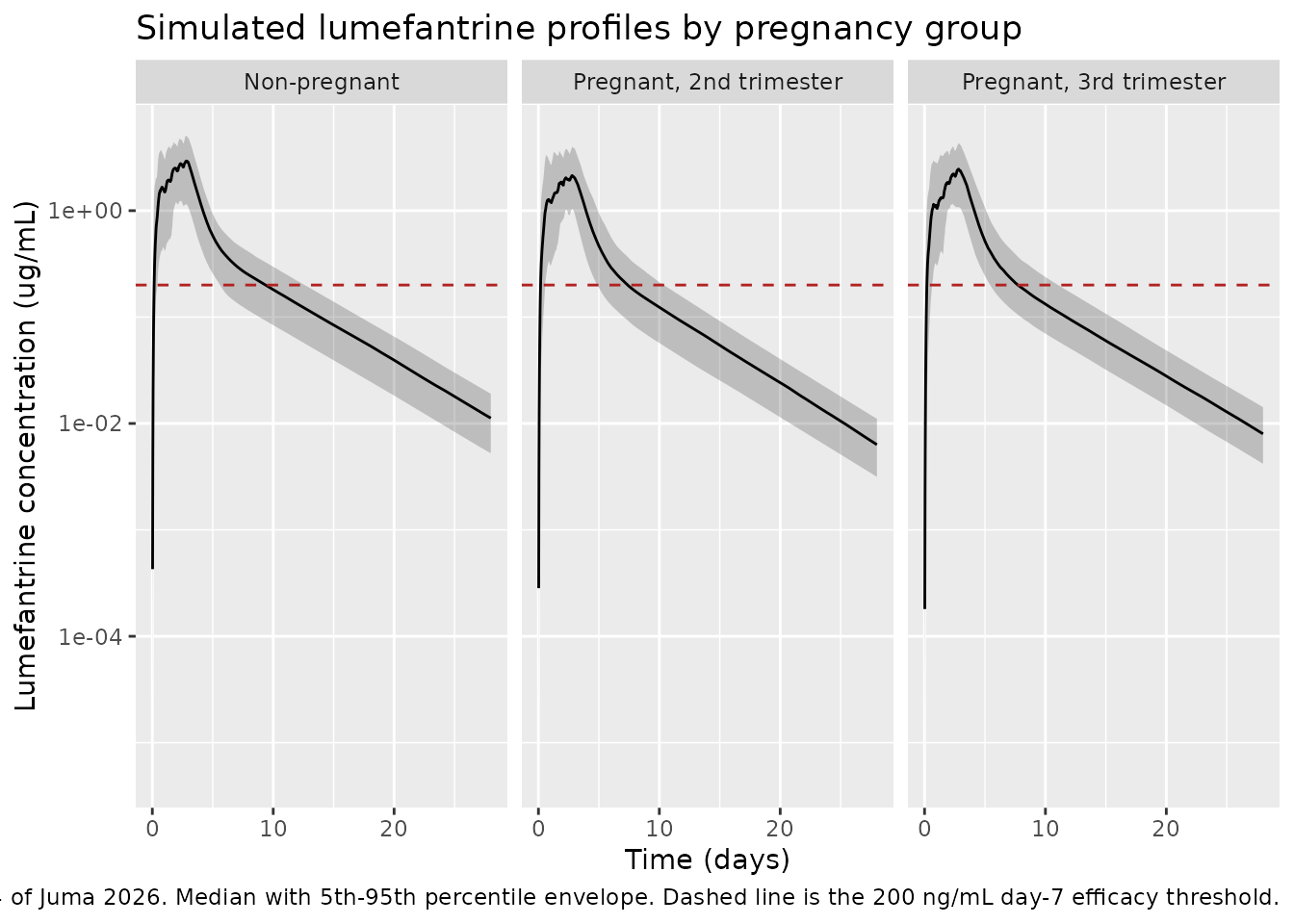
# Replicates Figure 4 of Juma 2026: predicted lumefantrine concentration-time
# profiles in non-pregnant (panel A) and pregnant (panel B) women. The paper's
# figure is a visual predictive check against observed data; the equivalent
# here is the simulated 5th / 50th / 95th percentile envelope.
sim |>
  dplyr::group_by(cohort, time) |>
  dplyr::summarise(
    Q05 = quantile(Cc, 0.05),
    Q50 = median(Cc),
    Q95 = quantile(Cc, 0.95),
    .groups = "drop"
  ) |>
  dplyr::filter(Q05 > 0) |>
  ggplot2::ggplot(ggplot2::aes(time / 24, Q50)) +
  ggplot2::geom_ribbon(ggplot2::aes(ymin = Q05, ymax = Q95), alpha = 0.25) +
  ggplot2::geom_line() +
  ggplot2::geom_hline(yintercept = 0.200, linetype = "dashed",
                      colour = "firebrick") +
  ggplot2::facet_wrap(~cohort) +
  ggplot2::scale_y_log10() +
  ggplot2::labs(
    x = "Time (days)", y = "Lumefantrine concentration (ug/mL)",
    title = "Simulated lumefantrine profiles by pregnancy group",
    caption = paste(
      "Replicates Figure 4 of Juma 2026. Median with 5th-95th percentile",
      "envelope. Dashed line is the 200 ng/mL day-7 efficacy threshold."
    )
  )
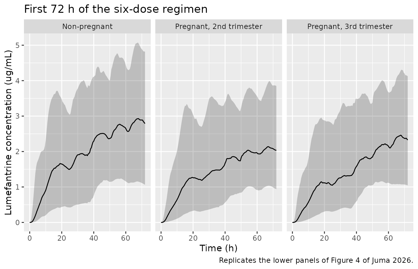
# The lower panels of Figure 4 zoom on the first 72 h of treatment.
sim |>
  dplyr::filter(time <= 72) |>
  dplyr::group_by(cohort, time) |>
  dplyr::summarise(
    Q05 = quantile(Cc, 0.05),
    Q50 = median(Cc),
    Q95 = quantile(Cc, 0.95),
    .groups = "drop"
  ) |>
  ggplot2::ggplot(ggplot2::aes(time, Q50)) +
  ggplot2::geom_ribbon(ggplot2::aes(ymin = Q05, ymax = Q95), alpha = 0.25) +
  ggplot2::geom_line() +
  ggplot2::facet_wrap(~cohort) +
  ggplot2::labs(
    x = "Time (h)", y = "Lumefantrine concentration (ug/mL)",
    title = "First 72 h of the six-dose regimen",
    caption = "Replicates the lower panels of Figure 4 of Juma 2026."
  )
PKNCA validation
sim_nca <- sim |>
  dplyr::filter(!is.na(Cc)) |>
  dplyr::select(id, time, Cc, cohort)

# Guarantee a pre-dose record so PKNCA can anchor AUC at time zero; for an
# oral model the correct pre-dose concentration is zero.
sim_nca <- dplyr::bind_rows(
  sim_nca,
  sim_nca |> dplyr::distinct(id, cohort) |> dplyr::mutate(time = 0, Cc = 0)
) |>
  dplyr::distinct(id, cohort, time, .keep_all = TRUE) |>
  dplyr::arrange(cohort, id, time)

conc_obj <- PKNCA::PKNCAconc(sim_nca, Cc ~ time | cohort + id)

dose_df <- events |>
  dplyr::filter(evid == 1) |>
  dplyr::select(id, time, amt, cohort)
dose_obj <- PKNCA::PKNCAdose(dose_df, amt ~ time | cohort + id)

# The paper's secondary parameters are for the whole six-dose course: Cmax is
# the peak over the regimen and AUC runs from time zero to infinity.
intervals <- data.frame(
  start      = 0,
  end        = Inf,
  cmax       = TRUE,
  tmax       = TRUE,
  auclast    = TRUE,
  aucinf.obs = TRUE,
  half.life  = TRUE
)

nca_res <- PKNCA::pk.nca(
  PKNCA::PKNCAdata(conc_obj, dose_obj, intervals = intervals)
)

nca_tbl <- as.data.frame(nca_res$result) |>
  dplyr::filter(PPTESTCD %in% c("cmax", "tmax", "aucinf.obs", "half.life")) |>
  dplyr::select(cohort, id, PPTESTCD, PPORRES)
stopifnot(nrow(nca_tbl) > 0, !anyNA(nca_tbl$PPORRES))

# Day-7 concentration is read directly off the simulation, not from PKNCA.
day7 <- sim |>
  dplyr::filter(abs(time - 168) < 1e-6) |>
  dplyr::transmute(cohort, id, PPTESTCD = "day7", PPORRES = Cc * 1000)

nca_all <- dplyr::bind_rows(nca_tbl, day7)
Comparison against the published secondary parameters
simulated <- nca_all |>
  dplyr::group_by(cohort, PPTESTCD) |>
  dplyr::summarise(median = median(PPORRES), .groups = "drop") |>
  tidyr::pivot_wider(names_from = PPTESTCD, values_from = median)

# Table 3 of Juma 2026, median (95% CI) across the Bayesian post-hoc estimates.
published <- tibble::tribble(
  ~cohort,                    ~half.life, ~cmax, ~aucinf.obs, ~day7,
  "Non-pregnant",             109,        3.21,  275,         277,
  "Pregnant, 2nd trimester",  103,        2.28,  184,         182,
  "Pregnant, 3rd trimester",  106,        2.44,  208,         192
)

cmp <- simulated |>
  dplyr::select(cohort, half.life, cmax, aucinf.obs, tmax, day7) |>
  dplyr::left_join(published, by = "cohort", suffix = c("_sim", "_pub")) |>
  dplyr::mutate(
    dplyr::across(dplyr::ends_with(c("_sim", "_pub")), ~ signif(.x, 3))
  )

cmp |>
  dplyr::select(
    cohort,
    half.life_sim, half.life_pub,
    cmax_sim, cmax_pub,
    aucinf.obs_sim, aucinf.obs_pub,
    day7_sim, day7_pub,
    tmax
  ) |>
  dplyr::rename(
    "Group"                    = cohort,
    "t1/2 sim (h)"             = half.life_sim,
    "t1/2 published (h)"       = half.life_pub,
    "Cmax sim (ug/mL)"         = cmax_sim,
    "Cmax published (ug/mL)"   = cmax_pub,
    "AUC sim (h*ug/mL)"        = aucinf.obs_sim,
    "AUC published (h*ug/mL)"  = aucinf.obs_pub,
    "Day 7 sim (ng/mL)"        = day7_sim,
    "Day 7 published (ng/mL)"  = day7_pub,
    "Tmax sim (h)"             = tmax
  ) |>
  knitr::kable(
    caption = paste(
      "Simulated versus published secondary PK parameters (Table 3 of",
      "Juma 2026). Simulated values are cohort medians; published values are",
      "medians of the Bayesian post-hoc estimates from the study cohorts.",
      "Tmax is not reported in the source."
    )
)| Group | t1/2 sim (h) | t1/2 published (h) | Cmax sim (ug/mL) | Cmax published (ug/mL) | AUC sim (h*ug/mL) | AUC published (h*ug/mL) | Day 7 sim (ng/mL) | Day 7 published (ng/mL) | Tmax sim (h) |
|---|---|---|---|---|---|---|---|---|---|
| Non-pregnant | 109 | 109 | 3.32 | 3.21 | 268 | 275 | 284 | 277 | 66.25 |
| Pregnant, 2nd trimester | 102 | 103 | 2.66 | 2.28 | 215 | 184 | 226 | 182 | 67.50 |
| Pregnant, 3rd trimester | 105 | 106 | 2.46 | 2.44 | 207 | 208 | 218 | 192 | 67.00 |
# Assert on the CENTRE of each cohort, never on its extremes: the extreme of a
# random cohort is not reproducible across rxode2 builds, whereas the median is
# driven by the structural parameters and the covariate model.
rel <- function(sim, pub) abs(sim - pub) / pub

chk <- cmp |>
  dplyr::transmute(
    cohort,
    hl   = rel(half.life_sim, half.life_pub),
    cmax = rel(cmax_sim, cmax_pub),
    auc  = rel(aucinf.obs_sim, aucinf.obs_pub),
    d7   = rel(day7_sim, day7_pub)
  )

stopifnot(
  # Terminal half-life is a pure function of the disposition parameters and is
  # essentially free of cohort noise, so it can carry a tight bound.
  all(chk$hl < 0.15),
  # Exposure medians compare a virtual cohort against post-hoc medians from the
  # real cohort, whose covariate distribution is only approximated here.
  all(chk$cmax < 0.30),
  all(chk$auc  < 0.35),
  all(chk$d7   < 0.35),
  # The non-pregnant arm is the model's reference group and its weight
  # distribution is the one reported directly in Table 1, so it is held to a
  # tighter bound than the two pregnant arms.
  chk$cmax[chk$cohort == "Non-pregnant"] < 0.20,
  chk$auc[chk$cohort == "Non-pregnant"]  < 0.20,
  chk$d7[chk$cohort == "Non-pregnant"]   < 0.20
)
round(chk[, -1] * 100, 1)
#>    hl cmax  auc   d7
#> 1 0.0  3.4  2.5  2.5
#> 2 1.0 16.7 16.8 24.2
#> 3 0.9  0.8  0.5 13.5
# Results 3.1.2 and the Discussion report that 44% of pregnant and 20% of
# non-pregnant women had a day-7 concentration below the 200 ng/mL threshold
# associated with therapeutic failure. Reproduced descriptively -- the source
# percentages come from the observed cohort of 50 and 25 women, so they are
# reported here rather than asserted on.
nca_all |>
  dplyr::filter(PPTESTCD == "day7") |>
  dplyr::group_by(cohort) |>
  dplyr::summarise(
    `Median day-7 (ng/mL)` = round(median(PPORRES)),
    `Below 200 ng/mL (%)`  = round(100 * mean(PPORRES < 200), 1),
    .groups = "drop"
  ) |>
  dplyr::rename("Group" = cohort) |>
  knitr::kable(
    caption = paste(
      "Day-7 lumefantrine concentrations against the 200 ng/mL efficacy",
      "threshold. Juma 2026 reports 44% of pregnant and 20% of non-pregnant",
      "women below this threshold."
    )
)| Group | Median day-7 (ng/mL) | Below 200 ng/mL (%) |
|---|---|---|
| Non-pregnant | 284 | 20.0 |
| Pregnant, 2nd trimester | 226 | 39.3 |
| Pregnant, 3rd trimester | 218 | 43.3 |
Assumptions and deviations
Allometric centring weight. Methods 2.11 states the allometric function “was centred on a typical body weight of 70 kg”, and the Table 2 note confirms that the population estimates are for a typical non-pregnant woman weighing 70 kg. The printed Equations 2 and 3 nevertheless write the denominator symbolically as
BW_median, and the study medians are 62.0 kg (pregnant) and 59.5 kg (non-pregnant). The model uses 70 kg, following the text and the Table 2 note.Transit chain length. Figure 1 draws a dose compartment transferring at
ktrinto a block ofn = 3transit compartments, which then transfers at a separately estimatedkainto the central compartment. The model therefore usesktr = 3 / MTT, i.e. MTT spans the threektr-governed transfers only, matching the convention of the co-author’smodellib("Ding_2024_amodiaquine")(2 transits,ktr = 2 / MTT, separateka). The alternative Savic-style readingktr = 4 / MTTwas tested against the published secondary parameters and is not distinguishable by them: because Cmax occurs after the last of six doses, the two readings differ by under 3% on median Cmax and under 2% on the day-7 concentration. No NONMEM control stream was available to settle the convention directly.Box-Cox transformed random effect on F. Results 3.1.2 describes the Box-Cox transformation as applying to the inter-individual variability of relative bioavailability, while Table 2 reports the single F variance term as inter-occasion variability (64.0% CV) and reports no separate F IIV row. The model encodes what Table 2 tabulates: one F variance term, carried across the two pooled dose occasions, with the Box-Cox shape
lambda = -0.690applied to it in the Petersson 2009 formeta_bc = (exp(lambda * eta) - 1) / lambda. Ateta = 0this returns 0 for anylambda, so the typical value of F is unaffected.No inter-individual variability on CL/F, Q/F or Vp/F. Equation 1 states that inter-individual variability was added exponentially to all PK parameters, but Table 2 of the final model reports variance terms only for MTT, Vc/F, ka and F. The model encodes the four terms that Table 2 reports; no variance is invented for the others. Almost all of the simulated exposure variability therefore arrives through the inter-occasion random effect on F.
Residual error scale. Methods 2.10 says residual variability was evaluated “as additive, proportional, or combined additive and proportional errors on log-transformed concentrations”, while Table 2 reports the retained combined model with a proportional term in per cent and an additive term in ng/mL, i.e. on the linear concentration scale. The model encodes
Cc ~ prop(propSd) + add(addSd)on the linear scale, with the additive term converted from 12.0 ng/mL to 0.0120 ug/mL to match the model’sug/mLconcentration unit.Gestational age was significant but is not encoded. Results 3.1.2 reports gestational age as a significant covariate on clearance (p < .01) and central volume (p < .05), but the model with binary pregnancy status had the lowest objective function value and was chosen as the final model; no gestational-age coefficient is printed. Gestational age is recorded in
covariatesDataExcludedrather than incovariateData.Dose50 value. Methods 2.11 fixes Dose50 at 3.84 mg/kg, “taken from a large pooled analysis of lumefantrine” (reference 8, Kloprogge 2018). The sibling model
modellib("Kloprogge_2018_lumefantrine")carries 3.86 mg/kg from its own Table 2. This model uses the 3.84 mg/kg value printed by Juma 2026.Body-weight summaries conflict between Table 1 and Results 3.1. Table 1 reports a non-pregnant median body weight of 59.5 kg (45.0-89.0), while Results 3.1 quotes “non-pregnant women [median 62 (range: 40-87)]” in the per-trimester comparison. The virtual cohort uses the Table 1 value for the non-pregnant arm and the Results 3.1 values for the two pregnant arms, which are given only there.
Virtual cohort covariates. Body weights are drawn log-normally around the published medians and truncated to the published ranges; the real joint distribution of weight, age and parasitaemia is not published. Age, baseline temperature and baseline parasitaemia were screened by the authors and not retained in the final model, so they are not simulated.
The 3rd-trimester versus 2nd-trimester ordering is not reproduced. Table 3 reports slightly higher Cmax and AUC in the third trimester than the second, whereas the model, whose only trimester-distinguishing input is body weight and whose allometry lowers exposure as weight rises, predicts the opposite ordering. The paper itself found no significant trimester effect, and the two published medians sit well inside each other’s confidence intervals, so this is a limitation of using body weight as a trimester proxy rather than a transcription discrepancy.
Desbutyl-lumefantrine is not modelled. The authors note this as a limitation of the study: the active metabolite was not measured and no metabolite model was built.