[212Pb]Pb-DOTAMTATE in vivo alpha generator whole-body PBPK in mice (Zaid 2021)
Source:vignettes/articles/Zaid_2021_pb212dotamtate_mouse_pbpk.Rmd
Zaid_2021_pb212dotamtate_mouse_pbpk.Rmd
library(nlmixr2lib)
library(rxode2)
library(PKNCA)
library(dplyr)
library(tidyr)
library(ggplot2)
library(knitr)
The model
Zaid et al. (Pharmaceutics 2021;13(12):2132, doi:10.3390/pharmaceutics13122132) built a whole-body physiologically based pharmacokinetic (PBPK) model of the in vivo alpha-particle generator [212Pb]Pb-DOTAMTATE, a somatostatin analogue that targets the sst2 receptor, in athymic nude mice bearing AR42J neuroendocrine tumour xenografts. The model follows the peptide and every radioactive daughter it produces, and uses them to compute absorbed doses.
mod <- rxode2::rxode2(nlmixr2lib::readModelDb("Zaid_2021_pb212dotamtate_mouse_pbpk"))
length(mod$state)
#> [1] 308
Seven species, two peptide systems
When 212Pb (half-life 10.6 h) beta-decays, the daughter 212Bi either
stays in the chelator, which gives [212Bi]Bi-DOTAMTATE, or, for the
fraction f = 0.16 of decays that populate an excited 212Bi
state, leaves it as free 212Bi. Free 212Bi binds to plasma proteins
(HWPP) and to red blood cells, and is taken up by tissue cells. The
alpha branch of 212Bi gives free 208Tl. 212Po, from the beta branch of
212Bi, decays within 0.3 microseconds and so deposits its 8.8 MeV alpha
energy where its parent decayed. The state names carry the species as a
prefix:
| Prefix | Species |
|---|---|
pb_ |
[212Pb]Pb-DOTAMTATE |
bis_ |
[212Bi]Bi-DOTAMTATE (chelated 212Bi) |
bi_, bihwpp_, birbc_
|
free 212Bi: unbound, bound to plasma proteins, bound to red cells |
tl_ |
free 208Tl |
cold_ |
unlabelled DOTAMTATE |
Unlabelled peptide is co-injected (the fitted study gave 0.0013 nmol, of which only 1.7e-5 nmol carried 212Pb), and every decay that strips the radionuclide from the peptide adds more. It competes with the labelled peptide for the same sst2 sites. The model therefore carries a second, unlabelled peptide system with the same physiology (Figure 2 of the paper).
Tissues
- sst2-expressing tissues (tumour, liver, spleen, pancreas, GI tract, adrenal, lung) have vascular, interstitial, receptor-bound, early-endosomal and sorting compartments (Figures 1 and 3). The bound complex is internalised at 0.17/min. From the early endosome it is either recycled to the interstitium (0.05/min) or routed to the sorting compartment (the fitted sorting rate).
- Kidneys bind the peptide from their vascular space, because the renal sst2 sites are on the glomerular podocytes. They also filter it into a proximal tubule, from which 98 % is excreted and the rest is taken up non-specifically.
- sst2-negative tissues (muscle, skin, heart, bone, fat, remainder of body) have a vascular and an interstitial compartment, plus a cellular compartment for free 212Bi.
- The brain is vascular-only and sits at arterial concentration.
- Spleen, pancreas and the GI tract drain into the liver.
Every state is an amount in nmol and time is in minutes.
cpb_<tissue> is the tissue concentration of
[212Pb]Pb-DOTAMTATE in nmol/g. Divided by the injected labelled amount
and multiplied by 100, it is the non-decay-corrected %ID/g of 212Pb that
the paper fitted. pbtot_, bistot_,
bitot_ and tltot_<tissue> are the tissue
amounts of each radionuclide, summed over the tissue’s sub-compartments.
They feed the dosimetry below.
Free receptors
The paper does not define the receptor term in its binding equations. The model takes free sst2 sites as the total sites minus every labelled and unlabelled complex that still holds a receptor. That includes complexes on the cell surface and complexes in early endosomes. The paper’s Methods describe the receptor travelling with the internalised complex and returning to the surface only after the complex dissociates in the endosome. The therapeutic-potency section shows that this reading, and not the surface-only definition of the framework paper (Kletting 2016, Eq 1), reproduces the optimal injected amounts of Figure 5.
Population
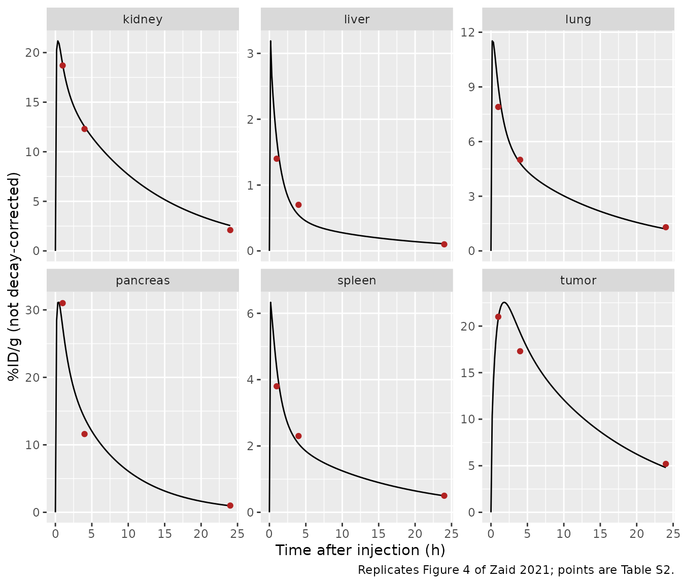
The model describes one standard 30 g mouse; it has no covariates and no between-animal variability. Every volume and flow in Table S1 is a literature fraction of body weight. The tumour is 300 uL, which the paper calls the tumour volume of the fitted study. The fitted data are the mean non-decay-corrected %ID/g in the kidneys, liver, spleen, pancreas, tumour and lung at 1, 4 and 24 h after 185 kBq (0.0013 nmol) of [212Pb]Pb-DOTAMTATE, as reported for AR42J tumour-bearing athymic nude mice by Stallons et al. (Mol Cancer Ther 2019). That source is reproduced in the paper’s Table S2. The number of animals per time point is not given.
Source trace
| Quantity | Source |
|---|---|
| sst2 densities (kidneys 3.52, liver 0.16, spleen 0.73, lung 1.77, pancreas 6.18, tumour 11.73 nmol/L), tumour perfusion 0.09 mL/min/g, sorting rate 0.0076/min, release rates (pancreas 0.0011, kidneys 0.000380 /min) | Table 1 (SimBiology column; SAAM II gives liver 0.17) |
| k_off 0.04/min, K_D 1 nmol/L, internalisation 0.17/min, recycling 0.05/min, release 0 in other tissues | Table S1; Methods 2.1 |
| Decay rates (212Pb 0.00109, 212Bi beta 0.00732, 212Bi alpha 0.00412, 208Tl 0.2236 /min) and dissociation fraction f = 0.16 | Table S1 |
| Free 212Bi binding to red cells (0.01, 0.017 /min) and HWPP (0.20, 0.20 /min) | Table S1 |
| Free 212Bi cellular uptake rates by tissue | Table S1 (tumour and adrenal not tabulated; see Assumptions) |
| Permeability-surface densities (muscle 0.02 peptide / 0.22 free nuclide; multipliers 500 / 100 / 1; tumour 0.31 mL/min/g) | Table S1 |
| GFR 0.0001 L/min, sieving 0.97 / 1, excretion fraction 0.98 / 0, tubule volume 0.1449 mL, tubular uptake 0.03/min | Table S1; Methods 2.1 |
| Body weight 30 g, haematocrit 0.45, red-cell scaling 0.86, organ, vascular, red-cell and interstitial fractions, flow fractions, cardiac output 0.275 BW^0.75 | Table S1 |
| sst2-expressing tissue ODEs (vascular, interstitial, bound, endosome, sorting) | Supplement A, Eqs 1-24 |
| Free 212Bi and 208Tl in blood and tissue | Supplement A, Eqs 25-38 |
| Kidney ODEs (vascular, bound, endosome, sorting, tubule, non-specific uptake, urine) | Supplement A, Eqs 39-64 |
| Arterial and venous pools; unlabelled peptide system | Reconstructed from Figures 1-2 by flow balance (see Assumptions) |
| Remainder-of-body flow and red-cell volume | Zaid 2021 rat 212Bi PBPK (Cancer Biother Radiopharm), Table A1 |
| Decay energies (212Pb beta 0.57, 212Bi beta 2.2, 212Bi alpha 6.1, 212Po alpha 8.8, 208Tl beta 1.8 MeV) and the MIRD dose formula | Table S1; Methods 2.3 |
| Fitted biodistribution (validation target) | Table S2 |
| Tumour-free predictions (validation target) | Supplement E, Table S3 |
| Absorbed-dose coefficients and per-nuclide contributions (validation target) | Table 2 |
| Optimal injected amounts at a fixed 23 Gy kidney dose (validation target) | Results; Figure 5 |
| Glomerular and tubular energy shares (validation target) | Results; Figure 6 |
Dosing helpers
A [212Pb]Pb-DOTAMTATE injection is a labelled dose into
pb_ven and the remaining, unlabelled, peptide into
cold_ven. The non-generator comparator,
[212Bi]Bi-DOTAMTATE, is dosed into bis_ven instead.
Observation rows sit on a real ODE state; every output is an algebraic
variable that rxode2 returns on every row.
th <- setNames(mod$iniDf$est, mod$iniDf$name)
lam_pb <- th[["lam_pb"]]
lam_bib <- th[["lam_bib"]]
lam_bia <- th[["lam_bia"]]
lam_tl <- th[["lam_tl"]]

# Labelled amount (nmol) carrying 185 kBq of 212Pb: A / lambda / N_A.
lab_fit <- 185e3 / (lam_pb / 60) / 6.02214076e23 * 1e9
total_fit <- 0.0013

dose_rows <- function(id, total, labelled, cmt) {
  data.frame(
    id = id, time = 0, evid = 1,
    amt = c(labelled, total - labelled),
    cmt = c(cmt, "cold_ven")
  )
}
make_events <- function(id, total, labelled, times, cmt = "pb_ven") {
  rbind(
    dose_rows(id, total, labelled, cmt),
    data.frame(id = id, time = times, evid = 0, amt = 0, cmt = "pb_ven")
  )
}
fitted_tissues <- c("kidney", "liver", "spleen", "pancreas", "tumor", "lung")

# Tissue mass (g) = total tissue volume (L) at 1 g/mL. The tumour volume is a
# fixed ini() parameter; every other volume is derived in model() and returned
# as an output column.
tissue_mass_g <- function(sim, tissues) {
  vapply(tissues, function(x) {
    1000 * if (x == "tumor") th[["vtot_tumor"]] else sim[[paste0("vtot_", x)]][1]
  }, numeric(1))
}
Fitted biodistribution (replicates Figure 4 and Table S2)
grid <- sort(unique(c(seq(0, 1440, by = 10), 60, 240)))
sim_fit <- rxode2::rxSolve(
  mod,
  make_events(1L, total_fit, lab_fit, grid),
  returnType = "data.frame"
)
pid_fit <- sim_fit |>
  select(time, all_of(paste0("cpb_", fitted_tissues))) |>
  pivot_longer(-time, names_to = "tissue", names_prefix = "cpb_", values_to = "cpb") |>
  mutate(pid = 100 * cpb / lab_fit)

obs_s2 <- tribble(
  ~time, ~kidney, ~liver, ~spleen, ~pancreas, ~tumor, ~lung,
  60, 18.7, 1.4, 3.8, 31, 21, 7.9,
  240, 12.3, 0.7, 2.3, 11.6, 17.3, 5,
  1440, 2.1, 0.1, 0.5, 1, 5.2, 1.3
) |>
  pivot_longer(-time, names_to = "tissue", values_to = "observed")
ggplot(pid_fit, aes(time / 60, pid)) +
  geom_line() +
  geom_point(data = obs_s2, aes(y = observed), colour = "firebrick") +
  facet_wrap(~tissue, scales = "free_y") +
  labs(
    x = "Time after injection (h)", y = "%ID/g (not decay-corrected)",
    caption = "Replicates Figure 4 of Zaid 2021; points are Table S2."
  )
cmp_s2 <- obs_s2 |>
  inner_join(pid_fit, by = c("time", "tissue")) |>
  mutate(pct_diff = 100 * (pid / observed - 1))
stopifnot(nrow(cmp_s2) == 18)
cmp_s2 |>
  mutate(time = time / 60, pid = signif(pid, 3), pct_diff = round(pct_diff)) |>
  select(tissue, time, observed, pid, pct_diff) |>
  rename(
    Tissue = tissue, "Time (h)" = time, "Table S2 %ID/g" = observed,
    "Simulated %ID/g" = pid, "Difference (%)" = pct_diff
  ) |>
kable(caption = "Fitted biodistribution: simulation against Table S2.")| Tissue | Time (h) | Table S2 %ID/g | Simulated %ID/g | Difference (%) |
|---|---|---|---|---|
| kidney | 1 | 18.7 | 18.800 | 1 |
| liver | 1 | 1.4 | 1.700 | 21 |
| spleen | 1 | 3.8 | 4.360 | 15 |
| pancreas | 1 | 31.0 | 27.500 | -11 |
| tumor | 1 | 21.0 | 20.800 | -1 |
| lung | 1 | 7.9 | 9.020 | 14 |
| kidney | 4 | 12.3 | 12.500 | 2 |
| liver | 4 | 0.7 | 0.545 | -22 |
| spleen | 4 | 2.3 | 2.070 | -10 |
| pancreas | 4 | 11.6 | 14.000 | 21 |
| tumor | 4 | 17.3 | 19.300 | 12 |
| lung | 4 | 5.0 | 4.820 | -4 |
| kidney | 24 | 2.1 | 2.560 | 22 |
| liver | 24 | 0.1 | 0.109 | 9 |
| spleen | 24 | 0.5 | 0.498 | 0 |
| pancreas | 24 | 1.0 | 0.967 | -3 |
| tumor | 24 | 5.2 | 4.810 | -8 |
| lung | 24 | 1.3 | 1.200 | -7 |
The model is deterministic, so these numbers do not depend on a random draw. The median absolute difference is about 10 % and no point is off by more than 25 %. The largest gaps, each about 22 %, are the liver at 1 and 4 h, the pancreas at 4 h and the kidneys at 24 h. The paper reports the fit only graphically (Figure 4), so the fit residuals cannot be compared directly. A mis-transcribed sst2 density, perfusion or rate moves its tissue’s whole curve far outside this envelope.
Tumour-free mouse (replicates Table S3)
Supplement E predicts the biodistribution in a mouse without a tumour by setting the tumour perfusion to zero. A vanishing perfusion stands in for zero here, because the parameter is on the log scale. Table S3 matches the simulation once the simulation is decay-corrected. Supplement E’s text implies that correction, although the table does not say so.
s3_tissues <- c("kidney", "liver", "lung", "pancreas", "spleen", "gi")
sim_s3 <- rxode2::rxSolve(
  mod,
  make_events(1L, total_fit, lab_fit, c(240, 1440)),
  params = c(lfperf_tumor = log(1e-12)),
  returnType = "data.frame"
)
obs_s3 <- tribble(
  ~time, ~kidney, ~liver, ~lung, ~pancreas, ~spleen, ~gi,
  240, 17.3, 0.8, 6.8, 19.8, 2.9, 9.2,
  1440, 10.7, 0.6, 6.2, 4.9, 2.6, 2.3
) |>
  pivot_longer(-time, names_to = "tissue", values_to = "table_s3")
cmp_s3 <- sim_s3 |>
  select(time, all_of(paste0("cpb_", s3_tissues))) |>
  pivot_longer(-time, names_to = "tissue", names_prefix = "cpb_", values_to = "cpb") |>
  mutate(pid_dc = 100 * cpb / lab_fit * exp(lam_pb * time)) |>
  inner_join(obs_s3, by = c("time", "tissue")) |>
  mutate(
    pct_diff = 100 * (pid_dc / table_s3 - 1),
    deviation = time == 1440 & tissue %in% c("kidney", "gi")
  )
stopifnot(nrow(cmp_s3) == 12)
cmp_s3 |>
  mutate(time = time / 60, pid_dc = signif(pid_dc, 3), pct_diff = round(pct_diff)) |>
  select(tissue, time, table_s3, pid_dc, pct_diff, deviation) |>
  rename(
    Tissue = tissue, "Time (h)" = time, "Table S3 %ID/g" = table_s3,
    "Simulated %ID/g (decay-corrected)" = pid_dc, "Difference (%)" = pct_diff,
    "Known deviation" = deviation
  ) |>
kable(caption = "Tumour-free mouse: simulation against Table S3.")| Tissue | Time (h) | Table S3 %ID/g | Simulated %ID/g (decay-corrected) | Difference (%) | Known deviation |
|---|---|---|---|---|---|
| kidney | 4 | 17.3 | 17.600 | 2 | FALSE |
| liver | 4 | 0.8 | 0.766 | -4 | FALSE |
| lung | 4 | 6.8 | 6.760 | -1 | FALSE |
| pancreas | 4 | 19.8 | 19.700 | 0 | FALSE |
| spleen | 4 | 2.9 | 2.900 | 0 | FALSE |
| gi | 4 | 9.2 | 9.190 | 0 | FALSE |
| kidney | 24 | 10.7 | 13.200 | 23 | TRUE |
| liver | 24 | 0.6 | 0.559 | -7 | FALSE |
| lung | 24 | 6.2 | 6.210 | 0 | FALSE |
| pancreas | 24 | 4.9 | 4.980 | 2 | FALSE |
| spleen | 24 | 2.6 | 2.560 | -1 | FALSE |
| gi | 24 | 2.3 | 8.420 | 266 | TRUE |
Ten of the twelve values agree within 10 %. The two exceptions are both at 24 h:
- GI tract: 8.4 simulated against 2.3 printed. The printed value is reproduced only if the GI tract releases radioactivity at the fitted pancreas rate. Table S1 sets release to zero in every tissue except the pancreas and kidneys, and the Discussion says so too, so the model keeps zero.
- Kidneys: 13.2 against 10.7 (+23 %).
Peptide mass balance
Decay only moves peptide between the labelled and the unlabelled systems. Release from the sorting compartment is the only route out of the model other than urine, and urine is a state. With both fitted release rates switched off, the total peptide in all states must stay equal to the injected amount.
Absorbed-dose coefficients (replicates Table 2)
Following the paper’s MIRD formula (Methods 2.3), the energy
deposited in a tissue is the time-integrated amount of each radionuclide
in it, times its decay rate and its energy per decay. The integration
runs from 0 to 10 half-lives of 212Pb (6384 min). Each 212Bi beta decay
also deposits the 8.8 MeV of the 212Po alpha decay that follows within
microseconds. The time-integrated amounts are the auclast
of each tissue amount, computed with PKNCA using the linear trapezoidal
rule. Tissue masses are the model’s total tissue volumes at 1 g/mL.
dose_end <- 6384
# 1-min steps while 212Bi-peptide (half-life 61 min) is distributing: the
# trapezoid then agrees with a 1-min grid over the whole range to 0.01 %, where
# a uniform 4-min grid overstates the 212Bi-peptide tumour dose by 1.3 %.
dose_grid <- c(seq(0, 120, by = 1), seq(122, 1440, by = 4), seq(1450, dose_end, by = 15))
tia <- function(long) {
  # Once an amount has decayed away the ODE solver can undershoot zero by a
  # rounding-level amount. Check the undershoot is noise, then floor it.
  undershoot <- long |>
    group_by(scenario, tissue, series, id) |>
    summarise(worst = min(amount) / max(abs(amount), 1e-300), .groups = "drop")
  stopifnot(all(undershoot$worst > -1e-4))
  long <- mutate(long, amount = pmax(amount, 0))
  conc <- PKNCA::PKNCAconc(long, amount ~ time | scenario + tissue + series / id)
  # No dose is supplied: only the AUC of tissue amounts is needed.
  dat <- suppressMessages(PKNCA::PKNCAdata(
    conc,
    intervals = data.frame(start = 0, end = dose_end, auclast = TRUE),
    options = list(auc.method = "linear")
  ))
  as.data.frame(suppressMessages(PKNCA::pk.nca(dat))) |>
    filter(PPTESTCD == "auclast") |>
    select(scenario, tissue, series, id, auc = PPORRES)
}
adc_tissues <- c(
  "tumor", "kidney", "pancreas", "liver", "lung", "spleen", "adrenal", "gi",
  "skin", "bone", "muscle", "heart", "brain", "fat", "rb"
)
sim_t2 <- rxode2::rxSolve(
  mod,
  make_events(1L, total_fit, lab_fit, dose_grid),
  returnType = "data.frame"
)
mass_g <- tissue_mass_g(sim_t2, adc_tissues)

long_t2 <- sim_t2 |>
  select(time, matches(paste0("^(pb|bis|bi|tl)tot_(", paste(adc_tissues, collapse = "|"), ")$"))) |>
  pivot_longer(-time, names_to = c("series", "tissue"), names_sep = "_", values_to = "amount") |>
  mutate(id = 1L, scenario = "Table 2")
auc_t2 <- tia(long_t2) |>
  pivot_wider(names_from = series, values_from = auc)
stopifnot(nrow(auc_t2) == length(adc_tissues))

# MeV x nmol per component; 212Po alpha follows every 212Bi beta decay.
energy_t2 <- auc_t2 |>
  transmute(
    tissue,
    pb_beta = 0.57 * lam_pb * pbtot,
    cbi_beta = 2.2 * lam_bib * bistot,
    cbi_alpha = 6.1 * lam_bia * bistot,
    cpo_alpha = 8.8 * lam_bib * bistot,
    fbi_beta = 2.2 * lam_bib * bitot,
    ftl_beta = 1.8 * lam_tl * tltot,
    fbi_alpha = 6.1 * lam_bia * bitot,
    fpo_alpha = 8.8 * lam_bib * bitot
  )
# ADC (Gy/MBq): energy (MeV) / A0 (Bq) / mass (kg). The nmol in the energy and
# the activity cancel; A0 = lambda_Pb (1/s) x labelled amount.
mev_to_j <- 1.602176634e-13
adc_t2 <- energy_t2 |>
  mutate(
    total = rowSums(across(pb_beta:fpo_alpha)),
    adc = total / (lam_pb / 60 * lab_fit) * mev_to_j / (mass_g[tissue] / 1000) * 1e6,
    across(pb_beta:fpo_alpha, ~ 100 * .x / total)
  )

paper_t2 <- tribble(
  ~tissue, ~adc_paper, ~pb_beta, ~cbi_beta, ~cbi_alpha, ~cpo_alpha, ~fbi_beta, ~ftl_beta, ~fbi_alpha, ~fpo_alpha,
  "tumor", 248, 5, 11, 18, 45, 2, 6, 3, 8,
  "kidney", 134, 6, 11, 18, 45, 2, 6, 3, 8,
  "pancreas", 116, 6, 11, 17, 44, 2, 6, 4, 9,
  "liver", 9, 5, 9, 14, 35, 5, 6, 7, 19,
  "lung", 65, 6, 11, 18, 45, 2, 6, 3, 8,
  "spleen", 28, 6, 11, 17, 44, 2, 6, 4, 10,
  "adrenal", 89, 6, 11, 18, 45, 2, 6, 3, 9,
  "gi", 85, 5, 11, 18, 45, 2, 6, 3, 9,
  "skin", 1.8, 9, 11, 16, 42, 2, 6, 4, 9,
  "bone", 2.7, 3, 3, 5, 14, 10, 7, 16, 41,
  "muscle", 0.6, 11, 11, 18, 46, 1, 7, 2, 4,
  "heart", 3.6, 2, 14, 23, 58, 0, 1, 0, 1,
  "brain", 0.1, 12, 11, 17, 43, 2, 6, 3, 7,
  "fat", 1.0, 9, 9, 14, 36, 1, 28, 1, 3,
  "rb", 1.0, 11, 11, 18, 45, 1, 6, 2, 5
)
components <- c("pb_beta", "cbi_beta", "cbi_alpha", "cpo_alpha", "fbi_beta", "ftl_beta", "fbi_alpha", "fpo_alpha")
cmp_t2 <- adc_t2 |>
  select(tissue, adc, all_of(components)) |>
  pivot_longer(all_of(components), names_to = "component", values_to = "simulated") |>
  inner_join(
    paper_t2 |> pivot_longer(all_of(components), names_to = "component", values_to = "paper"),
    by = c("tissue", "component")
  )
stopifnot(nrow(cmp_t2) == 8 * length(adc_tissues))

cmp_t2 |>
  mutate(cell = sprintf("%.0f (%g)", simulated, paper)) |>
  select(tissue, component, cell) |>
  pivot_wider(names_from = component, values_from = cell) |>
  rename(
    Tissue = tissue, "212Pb beta" = pb_beta, "c-212Bi beta" = cbi_beta,
    "c-212Bi alpha" = cbi_alpha, "c-212Po alpha" = cpo_alpha,
    "f-212Bi beta" = fbi_beta, "f-208Tl beta" = ftl_beta,
    "f-212Bi alpha" = fbi_alpha, "f-212Po alpha" = fpo_alpha
  ) |>
  kable(caption = paste(
    "Contribution (%) of each radionuclide to the absorbed dose, simulated",
    "(Table 2 in parentheses); c- = conjugated, f- = free."
))| Tissue | 212Pb beta | c-212Bi beta | c-212Bi alpha | c-212Po alpha | f-212Bi beta | f-208Tl beta | f-212Bi alpha | f-212Po alpha |
|---|---|---|---|---|---|---|---|---|
| adrenal | 6 (6) | 11 (11) | 18 (18) | 45 (45) | 2 (2) | 6 (6) | 3 (3) | 8 (9) |
| bone | 4 (3) | 4 (3) | 6 (5) | 17 (14) | 9 (10) | 7 (7) | 15 (16) | 38 (41) |
| brain | 12 (12) | 11 (11) | 17 (17) | 45 (43) | 1 (2) | 7 (6) | 2 (3) | 5 (7) |
| fat | 11 (9) | 12 (9) | 18 (14) | 47 (36) | 1 (1) | 6 (28) | 1 (1) | 4 (3) |
| gi | 5 (5) | 11 (11) | 18 (18) | 45 (45) | 2 (2) | 6 (6) | 3 (3) | 9 (9) |
| heart | 12 (2) | 12 (14) | 18 (23) | 46 (58) | 1 (0) | 6 (1) | 1 (0) | 4 (1) |
| kidney | 6 (6) | 11 (11) | 17 (18) | 45 (45) | 2 (2) | 6 (6) | 4 (3) | 9 (8) |
| liver | 5 (5) | 9 (9) | 14 (14) | 36 (35) | 5 (5) | 6 (6) | 7 (7) | 18 (19) |
| lung | 6 (6) | 11 (11) | 18 (18) | 45 (45) | 2 (2) | 6 (6) | 3 (3) | 9 (8) |
| muscle | 12 (11) | 12 (11) | 18 (18) | 46 (46) | 1 (1) | 6 (7) | 2 (2) | 4 (4) |
| pancreas | 6 (6) | 11 (11) | 17 (17) | 45 (44) | 2 (2) | 6 (6) | 4 (4) | 9 (9) |
| rb | 11 (11) | 12 (11) | 18 (18) | 46 (45) | 1 (1) | 6 (6) | 2 (2) | 4 (5) |
| skin | 10 (9) | 11 (11) | 17 (16) | 43 (42) | 2 (2) | 6 (6) | 3 (4) | 9 (9) |
| spleen | 6 (6) | 11 (11) | 17 (17) | 44 (44) | 2 (2) | 6 (6) | 4 (4) | 9 (10) |
| tumor | 5 (5) | 11 (11) | 18 (18) | 46 (45) | 2 (2) | 6 (6) | 3 (3) | 8 (8) |
The contributions reproduce Table 2 within 2 percentage points in 12 of the 15 tissues, and within 3 points in bone. Two rows cannot be reproduced:
- Heart: Table 2 gives 58 % from conjugated 212Po and almost no free nuclide. Its ADC is also 6 times the muscle ADC, although heart and muscle share every kinetic parameter in Table S1.
- Fat: Table 2 gives 28 % from 208Tl, against 6-7 % in every other tissue.
The heart row would fit a heart that included the cardiac blood, which the model places in the arterial and venous pools. No reading of the fat row has been found.
ok_t2 <- cmp_t2 |> filter(!tissue %in% c("heart", "fat", "bone"))
stopifnot(
  max(abs(ok_t2$simulated - ok_t2$paper)) < 2.5,
  max(abs(cmp_t2$simulated[cmp_t2$tissue == "bone"] - cmp_t2$paper[cmp_t2$tissue == "bone"])) < 4
)
The absolute ADCs are a factor of 11.2-12.0 below Table 2 in 11 of the 15 tissues, for example tumour 21.4 against 248 Gy/MBq. The exceptions are the kidneys (10.2), the brain (printed to one digit), fat and heart. A factor that is the same in every tissue is a reporting scale (activity, mass or energy units) and not a kinetic difference. The paper does not give enough of the calculation to recover it. The table below therefore compares each tissue’s ADC relative to the tumour, which cancels any common factor.
adc_cmp <- adc_t2 |>
  select(tissue, adc) |>
  inner_join(paper_t2 |> select(tissue, adc_paper), by = "tissue") |>
  mutate(
    scale = adc_paper / adc,
    rel_sim = adc / adc[tissue == "tumor"],
    rel_paper = adc_paper / adc_paper[tissue == "tumor"],
    pct_diff = 100 * (rel_sim / rel_paper - 1)
  )
adc_cmp |>
  mutate(across(c(adc, scale), ~ signif(.x, 3)), across(c(rel_sim, rel_paper), ~ signif(.x, 2)), pct_diff = round(pct_diff)) |>
  rename(
    Tissue = tissue, "Simulated ADC (Gy/MBq)" = adc, "Table 2 ADC" = adc_paper,
    "Table 2 / simulated" = scale, "Simulated, relative to tumour" = rel_sim,
    "Table 2, relative to tumour" = rel_paper, "Difference (%)" = pct_diff
  ) |>
kable(caption = "Absorbed-dose coefficients against Table 2.")| Tissue | Simulated ADC (Gy/MBq) | Table 2 ADC | Table 2 / simulated | Simulated, relative to tumour | Table 2, relative to tumour | Difference (%) |
|---|---|---|---|---|---|---|
| adrenal | 7.72000 | 89.0 | 11.5 | 0.36000 | 0.3600 | 0 |
| bone | 0.24200 | 2.7 | 11.2 | 0.01100 | 0.0110 | 4 |
| brain | 0.00719 | 0.1 | 13.9 | 0.00034 | 0.0004 | -17 |
| fat | 0.06350 | 1.0 | 15.8 | 0.00300 | 0.0040 | -27 |
| gi | 7.33000 | 85.0 | 11.6 | 0.34000 | 0.3400 | 0 |
| heart | 0.06050 | 3.6 | 59.5 | 0.00280 | 0.0150 | -81 |
| kidney | 13.20000 | 134.0 | 10.2 | 0.62000 | 0.5400 | 14 |
| liver | 0.75200 | 9.0 | 12.0 | 0.03500 | 0.0360 | -3 |
| lung | 5.68000 | 65.0 | 11.5 | 0.26000 | 0.2600 | 1 |
| muscle | 0.05210 | 0.6 | 11.5 | 0.00240 | 0.0024 | 0 |
| pancreas | 10.20000 | 116.0 | 11.3 | 0.48000 | 0.4700 | 2 |
| rb | 0.08470 | 1.0 | 11.8 | 0.00390 | 0.0040 | -2 |
| skin | 0.15000 | 1.8 | 12.0 | 0.00700 | 0.0073 | -3 |
| spleen | 2.44000 | 28.0 | 11.5 | 0.11000 | 0.1100 | 1 |
| tumor | 21.40000 | 248.0 | 11.6 | 1.00000 | 1.0000 | 0 |
main_organs <- adc_cmp |> filter(tissue %in% c("kidney", "pancreas", "liver", "lung", "spleen", "adrenal", "gi"))
stopifnot(
  abs(median(main_organs$pct_diff)) < 5,
  max(abs(main_organs$pct_diff)) < 20
)
Relative to the tumour, the sst2-expressing organs agree within a few percent, except the kidneys, which are about 14 % high. Equivalently, the simulated tumour-to-kidney ADC ratio is about 12 % below Table 2’s 248/134. That ratio caps the 212Pb tumour dose in the next section.
Therapeutic potency at a fixed kidney dose (replicates Figures 5 and 6)
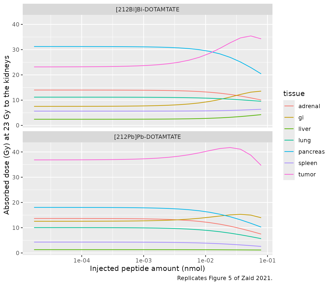
The paper swept the injected peptide amount from 0.017e-3 to 0.079 nmol in steps of 10^(1/6). At each amount it scaled the injected activity so that the kidneys received 23 Gy, then compared the resulting tumour dose with the same sweep for [212Bi]Bi-DOTAMTATE. Labelled and unlabelled peptide share every kinetic parameter, so at a fixed total amount the labelled distribution is exactly proportional to the labelled dose. The tissue dose at 23 Gy to the kidneys is therefore 23 Gy times the tissue’s energy per gram divided by the kidneys’ energy per gram. That ratio does not depend on the activity or on the absolute ADC scale. Each amount is simulated with a labelled fraction of 1e-6.
amounts <- 0.017e-3 * 10^((0:22) / 6)
tracers <- c(pb_ven = "[212Pb]Pb-DOTAMTATE", bis_ven = "[212Bi]Bi-DOTAMTATE")
dose_tissues <- c("tumor", "kidney", "pancreas", "lung", "adrenal", "gi", "spleen", "liver")
# Energy deposition rate (MeV x nmol / min) from every radionuclide in a tissue.
energy_rate <- function(pb, bis, bi, tl) {
  0.57 * lam_pb * pb + (bis + bi) * ((2.2 + 8.8) * lam_bib + 6.1 * lam_bia) + 1.8 * lam_tl * tl
}
# Glomeruli: renal vascular, bound, endosomal and sorting compartments.
# Proximal tubules: tubule lumen and the non-specific uptake compartment.
kidney_energy <- function(sim, subs) {
  pick <- function(sp) {
    cols <- intersect(paste0(sp, "_", subs, "_kidney"), names(sim))
    if (length(cols) == 0) {
      return(0)
    }
    rowSums(sim[, cols, drop = FALSE])
  }
  energy_rate(pick("pb"), pick("bis"), pick("bi") + pick("bihwpp") + pick("birbc"), pick("tl"))
}
# One solve per tracer, 23 amounts each, reduced at once to energy-rate series.
potency_long <- function(model, cmt) {
  events <- bind_rows(lapply(seq_along(amounts), function(i) {
    make_events(i, amounts[i], 1e-6 * amounts[i], dose_grid, cmt)
  }))
  sim <- rxode2::rxSolve(model, events, returnType = "data.frame")
  stopifnot(nrow(sim) == length(amounts) * length(dose_grid))
  bind_rows(
    lapply(dose_tissues, function(x) {
      data.frame(
        id = sim$id, time = sim$time, tissue = x, series = "energy",
        amount = energy_rate(
          sim[[paste0("pbtot_", x)]], sim[[paste0("bistot_", x)]],
          sim[[paste0("bitot_", x)]], sim[[paste0("tltot_", x)]]
        )
      )
    }),
    data.frame(
      id = sim$id, time = sim$time, tissue = "kidney", series = "glomeruli",
      amount = kidney_energy(sim, c("v", "bnd", "endo", "sort"))
    ),
    data.frame(
      id = sim$id, time = sim$time, tissue = "kidney", series = "tubules",
      amount = kidney_energy(sim, c("tub", "nsp"))
    )
  ) |>
    mutate(id = as.integer(as.character(id)))
}
potency <- function(model, label) {
  bind_rows(lapply(names(tracers), function(cmt) {
    potency_long(model, cmt) |>
      mutate(scenario = label) |>
      tia() |>
      mutate(
        tracer = tracers[[cmt]],
        amount_nmol = amounts[as.integer(as.character(id))]
      )
  }))
}
to_doses <- function(auc, mass) {
  auc |>
    filter(series == "energy") |>
    mutate(per_g = auc / mass[tissue]) |>
    group_by(scenario, tracer, amount_nmol) |>
    mutate(dose_gy = 23 * per_g / per_g[tissue == "kidney"]) |>
    ungroup()
}
mass_dose <- tissue_mass_g(sim_t2, dose_tissues)
auc_b <- potency(mod, "free = total - surface - endosomal")
doses_b <- to_doses(auc_b, mass_dose)
stopifnot(nrow(doses_b) == 2 * length(amounts) * length(dose_tissues))
doses_b |>
  filter(tissue != "kidney") |>
  ggplot(aes(amount_nmol, dose_gy, colour = tissue)) +
  geom_line() +
  scale_x_log10() +
  facet_wrap(~tracer, ncol = 1) +
  labs(
    x = "Injected peptide amount (nmol)", y = "Absorbed dose (Gy) at 23 Gy to the kidneys",
    caption = "Replicates Figure 5 of Zaid 2021."
  )
optimum <- function(doses) {
  doses |>
    filter(tissue == "tumor") |>
    group_by(scenario, tracer) |>
    slice_max(dose_gy, n = 1) |>
    ungroup() |>
    select(scenario, tracer, amount_nmol, dose_gy)
}
opt_b <- optimum(doses_b) |>
  left_join(
    tribble(
      ~tracer, ~paper_amount, ~paper_dose,
      "[212Pb]Pb-DOTAMTATE", 0.03, 49.8,
      "[212Bi]Bi-DOTAMTATE", 0.05, 36.6
    ),
    by = "tracer"
  )
opt_b |>
  mutate(amount_nmol = signif(amount_nmol, 2), dose_gy = round(dose_gy, 1)) |>
  select(tracer, amount_nmol, paper_amount, dose_gy, paper_dose) |>
  rename(
    Tracer = tracer, "Optimal amount (nmol)" = amount_nmol,
    "Paper optimum (nmol)" = paper_amount, "Tumour dose (Gy)" = dose_gy,
    "Paper tumour dose (Gy)" = paper_dose
  ) |>
kable(caption = "Tumour-dose optimum at a fixed 23 Gy kidney dose.")| Tracer | Optimal amount (nmol) | Paper optimum (nmol) | Tumour dose (Gy) | Paper tumour dose (Gy) |
|---|---|---|---|---|
| [212Bi]Bi-DOTAMTATE | 0.054 | 0.05 | 35.4 | 36.6 |
| [212Pb]Pb-DOTAMTATE | 0.025 | 0.03 | 41.7 | 49.8 |
pb_opt <- opt_b[opt_b$tracer == "[212Pb]Pb-DOTAMTATE", ]
bi_opt <- opt_b[opt_b$tracer == "[212Bi]Bi-DOTAMTATE", ]
stopifnot(
  nrow(pb_opt) == 1, nrow(bi_opt) == 1,
  # Both optima are interior and within one grid step of the paper's amount.
  pb_opt$amount_nmol < max(amounts), bi_opt$amount_nmol < max(amounts),
  abs(log10(pb_opt$amount_nmol / 0.03)) < 1.5 / 6,
  abs(log10(bi_opt$amount_nmol / 0.05)) < 1.5 / 6,
  # The generator beats the non-generator at its optimum (the paper's conclusion).
  pb_opt$dose_gy > bi_opt$dose_gy,
  abs(bi_opt$dose_gy / 36.6 - 1) < 0.05
)
Both optimal amounts are reproduced to within one step of the sweep. At its optimum, [212Bi]Bi-DOTAMTATE gives about 35 Gy, against the printed 36.6 Gy. [212Pb]Pb-DOTAMTATE gives about 42 Gy, against the printed 49.8 Gy. The tumour-to-kidney ADC ratio explains the gap: at the fitted amount it is about 12 % below Table 2’s 248/134, and the potency curve scales with that ratio. The generator therefore still delivers more tumour dose than the non-generator, but by less than the paper reports.
The free-receptor definition decides the optimum
The framework paper (Kletting 2016, Eq 1) defines free receptors as the total minus the surface-bound complexes only. Rebuilding the model with that definition, and changing nothing else, leaves the fitted biodistribution of Table S2 within 3 % of the model above. It does change the potency sweep: the tumour dose of both tracers then keeps rising up to the largest amount, so neither has an optimum.
mod_a <- mod |>
  rxode2::model(rfree_tumor <- rdens_tumor * vtot_tumor - pb_bnd_tumor - bis_bnd_tumor - cold_bnd_tumor) |>
  rxode2::model(rfree_liver <- rdens_liver * vtot_liver - pb_bnd_liver - bis_bnd_liver - cold_bnd_liver) |>
  rxode2::model(rfree_spleen <- rdens_spleen * vtot_spleen - pb_bnd_spleen - bis_bnd_spleen - cold_bnd_spleen) |>
  rxode2::model(rfree_pancreas <- rdens_pancreas * vtot_pancreas - pb_bnd_pancreas - bis_bnd_pancreas - cold_bnd_pancreas) |>
  rxode2::model(rfree_gi <- rdens_gi * vtot_gi - pb_bnd_gi - bis_bnd_gi - cold_bnd_gi) |>
  rxode2::model(rfree_adrenal <- rdens_adrenal * vtot_adrenal - pb_bnd_adrenal - bis_bnd_adrenal - cold_bnd_adrenal) |>
  rxode2::model(rfree_lung <- rdens_lung * vtot_lung - pb_bnd_lung - bis_bnd_lung - cold_bnd_lung) |>
  rxode2::model(rfree_kidney <- rdens_kidney * vtot_kidney - pb_bnd_kidney - bis_bnd_kidney - cold_bnd_kidney)

# The fitted biodistribution barely moves ...
fit_a <- rxode2::rxSolve(mod_a, make_events(1L, total_fit, lab_fit, c(60, 240, 1440)), returnType = "data.frame")
fit_b <- sim_fit[sim_fit$time %in% c(60, 240, 1440), ]
fit_shift <- max(abs(
  as.matrix(fit_a[, paste0("cpb_", fitted_tissues)]) /
    as.matrix(fit_b[, paste0("cpb_", fitted_tissues)]) - 1
))
fit_shift
#> [1] 0.02722808
# ... but the optimum disappears.
auc_a <- potency(mod_a, "free = total - surface")
opt_a <- optimum(to_doses(auc_a, mass_dose))
bind_rows(opt_b |> select(scenario, tracer, amount_nmol, dose_gy), opt_a) |>
  mutate(amount_nmol = signif(amount_nmol, 2), dose_gy = round(dose_gy, 1)) |>
  rename(
    "Free receptors" = scenario, Tracer = tracer,
    "Optimal amount (nmol)" = amount_nmol, "Tumour dose (Gy)" = dose_gy
  ) |>
kable(caption = "Tumour-dose optimum under the two free-receptor definitions.")| Free receptors | Tracer | Optimal amount (nmol) | Tumour dose (Gy) |
|---|---|---|---|
| free = total - surface - endosomal | [212Bi]Bi-DOTAMTATE | 0.054 | 35.4 |
| free = total - surface - endosomal | [212Pb]Pb-DOTAMTATE | 0.025 | 41.7 |
| free = total - surface | [212Bi]Bi-DOTAMTATE | 0.079 | 33.7 |
| free = total - surface | [212Pb]Pb-DOTAMTATE | 0.079 | 42.4 |
glom_share <- bind_rows(auc_b, auc_a) |>
  filter(series %in% c("glomeruli", "tubules")) |>
  select(scenario, tracer, amount_nmol, series, auc) |>
  pivot_wider(names_from = series, values_from = auc) |>
  mutate(glomeruli_pct = 100 * glomeruli / (glomeruli + tubules))
ggplot(glom_share, aes(amount_nmol, glomeruli_pct, colour = tracer)) +
  geom_line() +
  geom_hline(yintercept = 54, linetype = "dashed") +
  scale_x_log10() +
  facet_wrap(~scenario, ncol = 1) +
  labs(
    x = "Injected peptide amount (nmol)", y = "Kidney energy released in the glomeruli (%)",
    caption = "Replicates Figure 6 of Zaid 2021; dashed line = 54 % reported at both optima."
  )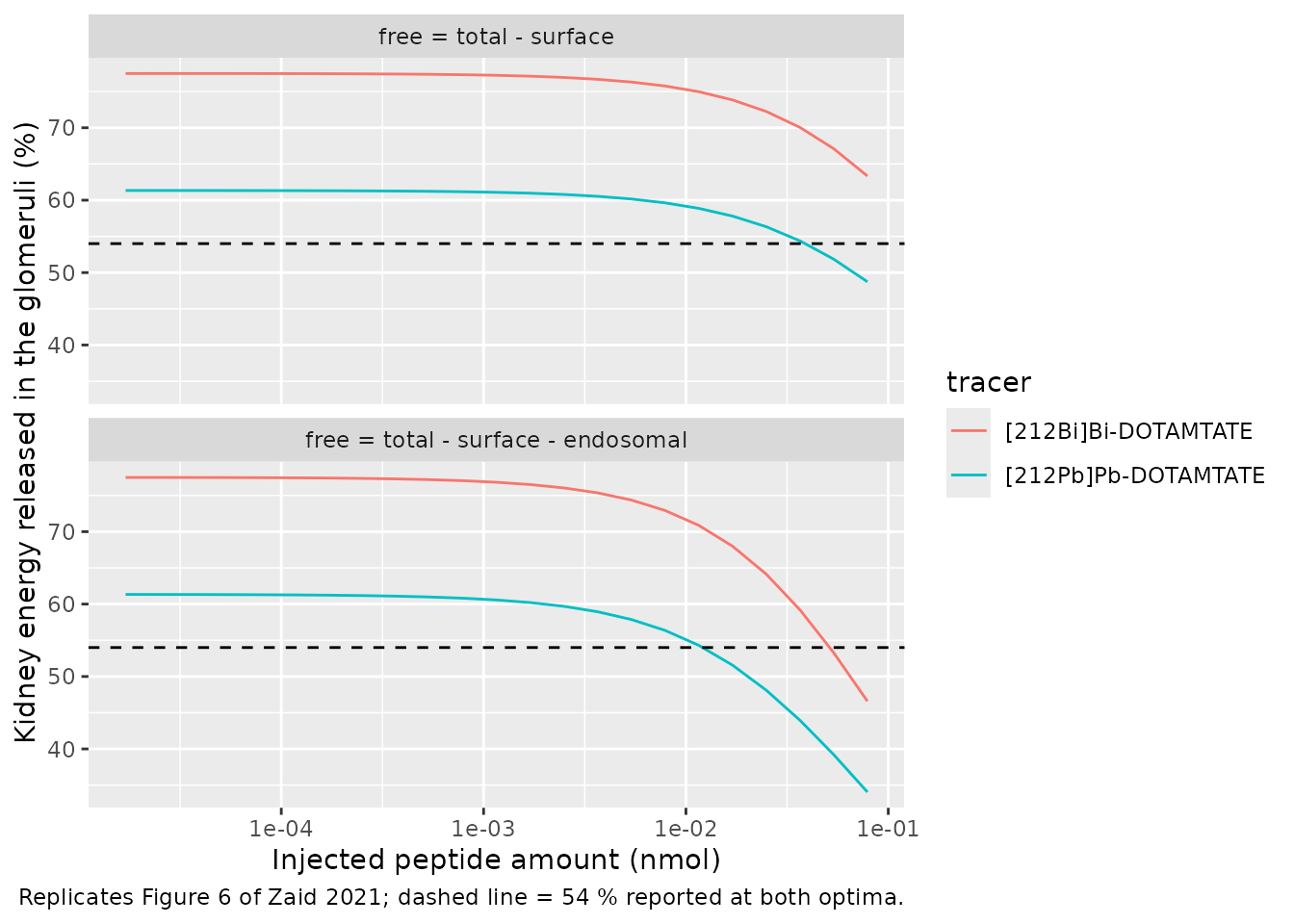
The paper reports that, at both optima, the glomeruli take 54 % and the proximal tubules 46 % of the energy absorbed in the kidneys. The table below reads the simulated glomerular share at the paper’s two optimal amounts, interpolated on the log-amount grid.
share_at <- function(tr, amt) {
  x <- glom_share |>
    filter(scenario == "free = total - surface - endosomal", tracer == tr)
  stopifnot(nrow(x) == length(amounts))
  stats::approx(log(x$amount_nmol), x$glomeruli_pct, xout = log(amt))$y
}
share_tab <- tibble(
  tracer = c("[212Bi]Bi-DOTAMTATE", "[212Pb]Pb-DOTAMTATE"),
  amount_nmol = c(0.05, 0.03),
  glomeruli_pct = c(share_at(tracer[1], amount_nmol[1]), share_at(tracer[2], amount_nmol[2])),
  paper_pct = 54
)
share_tab |>
  mutate(glomeruli_pct = round(glomeruli_pct)) |>
  rename(
    Tracer = tracer, "Amount (nmol)" = amount_nmol,
    "Simulated glomeruli share (%)" = glomeruli_pct, "Paper (%)" = paper_pct
  ) |>
kable(caption = "Share of the kidney energy released in the glomeruli at the paper's optima.")| Tracer | Amount (nmol) | Simulated glomeruli share (%) | Paper (%) |
|---|---|---|---|
| [212Bi]Bi-DOTAMTATE | 0.05 | 54 | 54 |
| [212Pb]Pb-DOTAMTATE | 0.03 | 46 | 54 |
The model reproduces the split for [212Bi]Bi-DOTAMTATE. For [212Pb]Pb-DOTAMTATE it puts slightly less than half of the kidney energy in the glomeruli, against the paper’s 54 %. As in the paper, the glomerular share falls as the amount grows and saturates the renal sst2 sites, and the short-lived [212Bi]Bi-DOTAMTATE releases more of its energy in the glomeruli.
Assumptions and deviations
The paper writes out the tissue equations (Supplement A, Eqs 1-64) and their parameters (Table S1), but not every part of the model. Each item below records how the model fills a gap or settles a conflict.
Reconstructed structure
-
Blood pools. The arterial and venous pools are not
written out.
- The arterial pool receives the lung outflow and feeds every perfused tissue.
- The venous pool collects every tissue outflow and receives the dose, and the portal organs return to it through the liver.
- Each pool holds its share of the serum plus half the cardiac serum, as in the same authors’ rat 212Bi PBPK.
-
Unlabelled peptide system. This system is described
only in prose and in Figure 2.
- It mirrors the labelled system.
- It gains unlabelled peptide in place from the decays that strip the radionuclide: 212Pb decays to excited 212Bi, and 212Bi-peptide decays.
- It shares the free sst2 sites with the labelled system.
- Free receptors. These are total sites minus surface-bound and early-endosomal complexes of both systems (see Free receptors and the reading comparison). The surface-only definition of Kletting 2016 Eq 1 fits Table S2 equally well but gives no optimum in Figure 5.
- Portal circulation. Spleen, pancreas and the GI tract drain into the liver, as Figure 1 draws, although Eq 1 has no portal term.
-
Remainder of body. Table S1 prints
f_RB = f_AdandV_RBC,RB = f_sc V_RBC,Ad. These are row copies that would leave about 13 % of cardiac output unaccounted for. The model instead uses the rat paper’s definitions:- remainder flow = cardiac output minus every other flow, the tumour included;
- remainder red-cell volume = total red-cell volume minus every tissue’s.
- Brain. Table S1 has no brain flow. The brain is vascular-only and is held at arterial concentration, which is the limit for any realistic flow.
- Free 212Bi in sst2-negative tissues. Table S1 gives these tissues cellular uptake rates, so they carry a cellular compartment, although the text lists only vascular and interstitial compartments.
- Stable 208Pb is not carried, because nothing depends on it.
Equation corrections (Supplement A)
- Eq 16: the 212Pb ground-state decay term is a loss; it is a gain.
- Eq 17: missing the cellular-uptake loss of free 212Bi.
- Eq 35: uses the red-cell dissociation rate for HWPP.
- Eq 37: omits the alpha decay of HWPP- and red-cell-bound 212Bi.
- Eq 40: binds 212Bi-peptide from the interstitium. The kidney has no interstitium, so it binds from the renal vascular space, as Eq 39 does for 212Pb-peptide.
- Eq 42: uses the total 212Pb decay rate for the ground-state branch.
- Eq 62: decays 212Bi-peptide instead of free 212Bi.
- Eq 63: excretes filtered 212Bi instead of 208Tl.
All of these were corrected by mass balance. Eq 38 and Eq 64 describe stable 208Pb, which the model does not carry. With release switched off, total peptide is conserved to solver precision (see Peptide mass balance).
Parameters not in Table S1
- Free-212Bi cellular uptake in the tumour and the adrenal is set to 0. Table 2 shows the tumour’s free-nuclide contributions equal to the kidneys’, and the model reproduces them.
- Free-nuclide permeability of the tumour is 3.41 mL/min/g. The maintainers derived it as the peptide value 0.31 times 11, because every tissue in Table S1 has a free-nuclide to peptide permeability ratio of 0.22/0.02 = 11.
Table conflicts kept as printed
- HWPP dissociation rate: 0.20/min as printed in Table S1. The cited rat paper reports 0.11/min, and 0.20/min is its association rate.
- Liver sst2 density: 0.16 nmol/L (SimBiology) rather than 0.17 (SAAM II). Table 2 and Figures 5-6 were computed in SimBiology.
-
Tumour red-cell volume:
v_t,v V_T H/(1-H), as printed in Table S1.
Outputs that do not reproduce
- Absolute ADCs. These are a factor of 11.2-12.0 below Table 2 in 11 of the 15 tissues. That is a reporting scale, and the paper does not give enough of the calculation to recover it. The comparisons above use relative ADCs and percentage contributions instead.
- Heart and fat in Table 2: see Absorbed-dose coefficients.
- Table S3 at 24 h: GI 8.4 against 2.3, and kidneys +23 %.
- [212Pb]Pb-DOTAMTATE in Figure 5: the peak tumour dose is about 42 Gy against 49.8 Gy, following from a tumour-to-kidney ADC ratio 12 % below Table 2’s.
- Figure 6: the 54/46 glomeruli/tubule split is reproduced for [212Bi]Bi-DOTAMTATE but not for [212Pb]Pb-DOTAMTATE (about 46/54).