Vancomycin (Stockmann 2015)
Source:vignettes/articles/Stockmann_2015_vancomycin.Rmd
Stockmann_2015_vancomycin.RmdModel and source
- Citation: Stockmann C, Hersh AL, Roberts JK, Bhongsatiern J, Korgenski EK, Spigarelli MG, Sherwin CMT, Frymoyer A. Predictive Performance of a Vancomycin Population Pharmacokinetic Model in Neonates. Infect Dis Ther. 2015;4(2):187-198. doi:10.1007/s40121-015-0067-9 (Methods, Model Evaluation: Equations 1 and 2 and the accompanying variance text). The structural model and every parameter estimate originate from Frymoyer A, Hersh AL, El-Komy MH, et al. Association Between Vancomycin Trough Concentration and AUC in Neonates. Antimicrob Agents Chemother. 2014 (cited as reference 7 of Stockmann 2015, whose reference list gives no volume, pages or DOI). Stockmann 2015 reprints the complete model, so no value here is taken from a source other than Stockmann 2015 itself.
- Description: One-compartment IV population PK model for vancomycin in neonates, as implemented and externally validated by Stockmann 2015. Clearance is driven by three covariates: allometric body weight (exponent 0.75, reference 2.9 kg), a sigmoidal postmenstrual-age maturation function (TM50 = 34.8 weeks, Hill = 4.53), and serum creatinine entering as (1/CREAT)^0.267 with CREAT in mg/dL on the Jaffe scale. Central volume scales linearly with weight (1.75 L at 2.9 kg). The structural and variance parameters were NOT estimated in Stockmann 2015; they are fixed priors carried verbatim from the originating model of Frymoyer 2014, which Stockmann 2015 re-implemented in NONMEM 7.2 and evaluated against an independent cohort of 243 neonates.
- Article: https://doi.org/10.1007/s40121-015-0067-9
Stockmann 2015 is an external validation paper. It estimated nothing: it re-implemented a previously published neonatal vancomycin population PK model in NONMEM 7.2 “with the structural and variance parameter values set equal to the estimates reported previously” and evaluated it against an independent cohort of 243 neonates. The originating model is Frymoyer 2014 (reference 7 of Stockmann 2015). Stockmann 2015 nonetheless reprints the model in full – Equations 1 and 2 give every structural constant, and the Methods text gives both inter-individual variances and both residual-error terms – so the extraction below is sourced entirely from Stockmann 2015 and no value is carried in from a publication that was not available when this model was built.
Population
The parameters were estimated from the model development cohort of 249 neonates described in the “Model development cohort” column of Stockmann 2015 Table 1 (whose footnote a attributes it to Frymoyer 2014): 49% female, gestational age median 34 weeks (range 23-42), body weight median 2.9 kg (range 0.5-6.3), postnatal age median 19 days (range 0-173), postmenstrual age median 39 weeks (range 24-53), and serum creatinine median 0.4 mg/dL (range 0.1-2.7) measured by the Jaffe method.
The 2.9 kg reference weight that appears in both Equations 1 and 2 is exactly this cohort’s median weight, which is a useful independent corroboration that both equations were transcribed correctly.
Stockmann 2015’s own contribution is the external validation cohort: 243 neonates contributing 734 vancomycin concentrations (mean 3.0 +/- 1.8 each) from five Intermountain Healthcare neonatal intensive care units between 2006 and 2013. It was lighter and less mature than the development cohort (weight median 1.6 kg, range 0.4-6.8; postmenstrual age median 33 weeks, range 23-54) and had higher serum creatinine (median 0.6 mg/dL, range 0.3-1.5). The median dose was 15.5 mg/kg (IQR 13.9-19.3) and the median dosing interval 11.5 h (IQR 8.0-12.5), administered as 1-h infusions (Table 2 heading).
The same information is available programmatically via the model’s
population metadata:
pop <- rxode2::rxode(readModelDb("Stockmann_2015_vancomycin"))$population
str(pop, max.level = 1)
#> List of 16
#>  $ species          : chr "human"
#>  $ n_subjects       : int 249
#>  $ n_studies        : int 1
#>  $ age_range        : chr "24-53 weeks postmenstrual age"
#>  $ age_median       : chr "39 weeks postmenstrual age"
#>  $ weight_range     : chr "0.5-6.3 kg"
#>  $ weight_median    : chr "2.9 kg"
#>  $ sex_female_pct   : num 49
#>  $ race_ethnicity   : chr "Not reported"
#>  $ disease_state    : chr "Neonates receiving intravenous vancomycin with therapeutic drug monitoring performed. Neonates with congenital "| __truncated__
#>  $ dose_range       : chr "Intravenous vancomycin as 1-h infusions per routine clinical practice. In the Stockmann 2015 validation cohort "| __truncated__
#>  $ regions          : chr "United States"
#>  $ ga_range         : chr "23-42 weeks gestational age (median 34)"
#>  $ renal_function   : chr "Serum creatinine median 0.4 mg/dL (range 0.1-2.7), Jaffe method"
#>  $ notes            : chr "DEVELOPMENT population, from the 'Model development cohort (n = 249)' column of Stockmann 2015 Table 1, whose f"| __truncated__
#>  $ validation_cohort: chr "Stockmann 2015's own contribution: 243 neonates with 734 vancomycin concentrations (mean 3.0 +/- 1.8 per neonat"| __truncated__
Source trace
Every ini() entry carries an in-file comment naming its
source location. They are collected here for review. Note that Equations
1 and 2 are typeset mathematics; the constants below were read from the
rendered equations in the PDF, because text extraction of this article
mangles the decimal points in the equation font (0.75 is
extracted as 0:75).
| Equation / parameter | Value | Source location |
|---|---|---|
lcl |
log(0.345) |
Equation 1, leading coefficient
CL (L/h) = 0.345 x ...
|
e_wt_cl |
0.75 |
Equation 1, exponent on (Weight / 2.9 kg)
|
pma_tm50 |
34.8 |
Equation 1, denominator of (PMA_weeks / 34.8)
|
pma_hill |
4.53 |
Equation 1, magnitude of the negative exponent
-4.53
|
e_creat_cl |
0.267 |
Equation 1, exponent on (1 / Cr_mg/dL)
|
lvc |
log(1.75) |
Equation 2, leading coefficient V (L) = 1.75 x ...
|
weight on vc
|
(WT / 2.9)^1 |
Equation 2 carries no exponent on
(Weight / 2.9 kg)
|
etalcl |
0.216^2 = 0.046656 |
Methods, Model Evaluation: exponential IIV on CL, “% CV 21.6%” |
etalvc |
0.109^2 = 0.011881 |
Methods, Model Evaluation: exponential IIV on V, “% CV 10.9%” |
propSd |
0.205 |
Methods, Model Evaluation: “combined proportional (% CV 20.5%)” |
addSd |
1.3 |
Methods, Model Evaluation: “additive error model (standard deviation +/- 1.3 mg/L)” |
d/dt(central) |
n/a | Methods, Model Evaluation: “a one compartment model with first-order elimination” |
| reference weight 2.9 kg | n/a | Table 1, model development cohort median weight |
| 1-h infusion | n/a | Table 2 heading, “relative to the end of the most recent 1-h infusion” |
Structural check against the printed equations
Before simulating anything, confirm that the compiled model reproduces Equations 1 and 2 when they are evaluated by hand at the development cohort’s median covariates (weight 2.9 kg, postmenstrual age 39 weeks, serum creatinine 0.4 mg/dL). The right-hand sides below are transcribed directly from the printed equations, independently of the model file, so a mis-typed constant in either place makes this check fail.
mod <- readModelDb("Stockmann_2015_vancomycin")

ref_wt <- 2.9    # kg,      Table 1 development-cohort median weight
ref_pma <- 39    # weeks,   Table 1 development-cohort median postmenstrual age
ref_cr <- 0.4    # mg/dL,   Table 1 development-cohort median serum creatinine

# Equation 1 and Equation 2, written out as printed.
cl_eq <- 0.345 * (ref_wt / 2.9)^0.75 *
  1 / (1 + (ref_pma / 34.8)^(-4.53)) *
  (1 / ref_cr)^0.267
vc_eq <- 1.75 * (ref_wt / 2.9)

# One typical subject, random effects zeroed, 15.5 mg/kg q12h at steady state.
tau <- 12
dose_mg <- 15.5 * ref_wt

typ_ev <- bind_rows(
  tibble(
    id = 1L, time = 0, amt = dose_mg, evid = 1L, cmt = "central",
    dur = 1, ii = tau, ss = 1L, addl = 24 / tau - 1
  ),
  tibble(
    id = 1L, time = seq(0, 24, by = 0.02), amt = NA_real_, evid = 0L,
    cmt = "central", dur = NA_real_, ii = 0, ss = 0L, addl = 0
  )
) |>
  mutate(WT = ref_wt, PAGE = ref_pma, CREAT = ref_cr) |>
  arrange(time, desc(evid))

# steady-state searches for long-half-life subjects exceed the default step budget
sim_typ <- rxode2::rxSolve(rxode2::zeroRe(mod), events = typ_ev,
                           maxsteps = 1e6) |>
  as.data.frame()
#> ℹ omega/sigma items treated as zero: 'etalcl', 'etalvc'

cl_mod <- sim_typ$cl[1]
vc_mod <- sim_typ$vc[1]

stopifnot(
  isTRUE(all.equal(cl_mod, cl_eq, tolerance = 1e-8)),
  isTRUE(all.equal(vc_mod, vc_eq, tolerance = 1e-8))
)

kel_typ <- cl_mod / vc_mod
tibble(
  Quantity = c("CL (L/h)", "V (L)", "kel (1/h)", "t1/2 (h)"),
  Value = c(cl_mod, vc_mod, kel_typ, log(2) / kel_typ)
) |>
knitr::kable(digits = 4, caption = "Typical values at the development-cohort median covariates.")| Quantity | Value |
|---|---|
| CL (L/h) | 0.2759 |
| V (L) | 1.7500 |
| kel (1/h) | 0.1577 |
| t1/2 (h) | 4.3959 |
The model reproduces both printed equations exactly.
Closed-form steady-state check
For a one-compartment model given as a Tinf-hour
infusion every tau hours, the steady-state concentration at
the end of the infusion and at the end of the interval have exact closed
forms. Comparing them to the ODE solve confirms the ss = 1
steady-state handling and the Cc = central / vc scaling.
Both sides use the same parameters, so this is a numerical-accuracy
gate, not a transcription gate – the transcription gate is the block
above.
t_inf <- 1
c_end_inf <- (dose_mg / (t_inf * cl_mod)) *
  (1 - exp(-kel_typ * t_inf)) / (1 - exp(-kel_typ * tau))
c_trough <- c_end_inf * exp(-kel_typ * (tau - t_inf))

obs_typ <- sim_typ |> filter(!is.na(Cc))
sim_cmax <- max(obs_typ$Cc)
sim_trough <- obs_typ$Cc[which.min(abs(obs_typ$time - 24))]

# Trapezoidal AUC over the full 24-h window (two complete intervals at steady
# state), and the identity the paper's Methods use: AUC24 = daily dose / CL.
auc24_trap <- with(obs_typ, sum(diff(time) * (head(Cc, -1) + tail(Cc, -1)) / 2))
auc24_id <- (dose_mg * 24 / tau) / cl_mod

cf <- tibble(
  Quantity = c("Cmax,ss (mg/L)", "Ctrough,ss (mg/L)", "AUC0-24 (mg*h/L)"),
  `Closed form` = c(c_end_inf, c_trough, auc24_id),
  `ODE solve` = c(sim_cmax, sim_trough, auc24_trap)
) |>
  mutate(`% diff` = 100 * (`ODE solve` - `Closed form`) / `Closed form`)

knitr::kable(cf, digits = 4, caption = "Closed-form steady state vs. the ODE solve.")| Quantity | Closed form | ODE solve | % diff |
|---|---|---|---|
| Cmax,ss (mg/L) | 27.9810 | 27.9810 | 0e+00 |
| Ctrough,ss (mg/L) | 4.9384 | 4.9384 | 1e-04 |
| AUC0-24 (mg*h/L) | 325.7932 | 325.7934 | 1e-04 |
Virtual cohort
The observed data are not publicly available. The cohort below approximates the covariate distributions of Stockmann 2015’s external validation cohort (Table 1): postmenstrual age median 33 weeks (range 23-54), weight median 1.6 kg (range 0.4-6.8), and Jaffe-standardized serum creatinine median 0.6 mg/dL (range 0.3-1.5). Weight and postmenstrual age are strongly coupled in neonates, so weight is generated from a log-linear growth curve in postmenstrual age rather than sampled independently – an independent draw would produce combinations such as 0.4 kg at 54 weeks that cannot occur.
The regimen is the cohort’s median reported regimen: 15.5 mg/kg as a 1-h infusion every 12 h at steady state. The paper’s median interval was 11.5 h; 12 h is the nearest clinically used interval and, unlike 11.5 h, divides 24 h evenly so that a 24-h window contains a whole number of dosing intervals. The sensitivity of the results to this choice is quantified below.
# set.seed() seeds R's RNG for the covariate draws. rxode2's own simulation RNG
# is partitioned per solver thread, so the realised cohort differs between a
# 2-thread CI runner and a 16-thread workstation. Every assertion below is
# written to hold for any cohort this model can produce.
set.seed(20150522)
rxode2::rxSetSeed(20150522)

n_sub <- 200

# Postmenstrual age: median 33 weeks, truncated to the observed 23-54 range.
pma <- pmin(pmax(rnorm(n_sub, 33.5, 6.5), 23), 54)

# Weight-for-postmenstrual-age. The log-linear segment is anchored on two points
# consistent with Table 1: about 0.55 kg at 23 weeks and about 3.4 kg at term
# (40 weeks); growth slows after term. Lognormal residual scatter, then truncated
# to the observed 0.4-6.8 kg range.
wt_med <- exp(-0.598 + 0.10715 * (pmin(pma, 40) - 23) + 0.035 * pmax(pma - 40, 0))
wt <- pmin(pmax(wt_med * exp(rnorm(n_sub, 0, 0.22)), 0.4), 6.8)

# Serum creatinine on the Jaffe scale: median 0.6 mg/dL, truncated to 0.3-1.5.
creat <- pmin(pmax(rlnorm(n_sub, log(0.6), 0.30), 0.3), 1.5)

subj <- tibble(
  id = seq_len(n_sub),
  WT = wt,
  PAGE = pma,
  CREAT = creat,
  amt_mg = 15.5 * wt
)

tibble(
  Covariate = c("Postmenstrual age (weeks)", "Weight (kg)", "Serum creatinine (mg/dL)"),
  `Simulated median` = c(median(subj$PAGE), median(subj$WT), median(subj$CREAT)),
  `Simulated range` = c(
    sprintf("%.0f-%.0f", min(subj$PAGE), max(subj$PAGE)),
    sprintf("%.1f-%.1f", min(subj$WT), max(subj$WT)),
    sprintf("%.1f-%.1f", min(subj$CREAT), max(subj$CREAT))
  ),
  `Table 1 median` = c(33, 1.6, 0.6),
  `Table 1 range` = c("23-54", "0.4-6.8", "0.3-1.5")
) |>
knitr::kable(digits = 2, caption = "Virtual cohort vs. Stockmann 2015 Table 1, external validation cohort.")| Covariate | Simulated median | Simulated range | Table 1 median | Table 1 range |
|---|---|---|---|---|
| Postmenstrual age (weeks) | 33.06 | 23-50 | 33.0 | 23-54 |
| Weight (kg) | 1.62 | 0.4-6.8 | 1.6 | 0.4-6.8 |
| Serum creatinine (mg/dL) | 0.60 | 0.3-1.2 | 0.6 | 0.3-1.5 |
dosing <- subj |>
  transmute(
    id, time = 0, amt = amt_mg, evid = 1L, cmt = "central",
    dur = 1, ii = tau, ss = 1L, addl = 24 / tau - 1
  )

# Observation rows use the ODE state name "central"; rxode2 returns the
# algebraic observable Cc as a column at those rows.
obs <- subj |>
  select(id) |>
  tidyr::crossing(time = seq(0, 24, by = 0.1)) |>
  mutate(
    amt = NA_real_, evid = 0L, cmt = "central",
    dur = NA_real_, ii = 0, ss = 0L, addl = 0
  )

events <- bind_rows(dosing, obs) |>
  left_join(subj |> select(id, WT, PAGE, CREAT, amt_mg), by = "id") |>
  arrange(id, time, desc(evid))

stopifnot(!anyDuplicated(unique(events[, c("id", "time", "evid")])))
Simulation
# The mass-balance identity below is gated at 1e-6 %, so both the ODE solve
# and its `ss = 1` steady-state search run at tight tolerances: at the
# defaults the steady-state search alone leaves ~1e-4 % of residual.
sim <- rxode2::rxSolve(
  mod, events = events, keep = c("amt_mg"),
  rtol = 1e-10, atol = 1e-12, ssRtol = 1e-10, ssAtol = 1e-12,
  # steady-state searches for long-half-life subjects exceed the default step budget
  maxsteps = 1e6
) |>
  as.data.frame()

sim_obs <- sim |> filter(!is.na(Cc))
stopifnot(nrow(sim_obs) > 0, all(sim_obs$Cc >= 0))

per_sub <- sim_obs |>
  group_by(id) |>
  summarise(
    cl = first(cl), vc = first(vc), amt_mg = first(amt_mg),
    trough = Cc[which.min(abs(time - 24))],
    cmax = max(Cc),
    auc24_trap = sum(diff(time) * (head(Cc, -1) + tail(Cc, -1)) / 2),
    .groups = "drop"
  ) |>
  mutate(
    daily_dose = amt_mg * 24 / tau,
    # The paper's Methods definition: "AUC24 was calculated as the daily dose / CL".
    auc24 = daily_dose / cl,
    thalf = log(2) * vc / cl
  )
Mass-balance identity
At steady state over a whole number of dosing intervals, the amount
entering equals the amount cleared, so AUC(0,24) x CL must
equal the 24-h dose exactly. This is the identity the paper’s Methods
use to compute AUC24, and it checks the ODE, the
Cc = central / vc scaling and the steady-state handling
together. Both sides derive from the same drawn parameters, so the
residual is pure numerical integration error and a tight bound is
correct.
per_sub <- per_sub |>
  mutate(auc_pct = 100 * (auc24_trap - auc24) / auc24)

# Realised max |% diff| was ~1e-12 at each of five seeds with the analytic
# solution, and ~5e-8 with the ODE integrated at rtol 1e-10 / ssRtol 1e-10;
# 1e-6 leaves headroom for either while still failing loudly on any scaling
# or steady-state error.
stopifnot(max(abs(per_sub$auc_pct)) < 1e-6)

sprintf(
  "AUC(0,24) x CL vs 24-h dose: median |%% diff| = %.2e, max |%% diff| = %.2e",
  median(abs(per_sub$auc_pct)), max(abs(per_sub$auc_pct))
)
#> [1] "AUC(0,24) x CL vs 24-h dose: median |% diff| = 3.97e-09, max |% diff| = 4.83e-08"
Replicate published figures
Figures 1 and 2 of Stockmann 2015 (observed-versus-predicted and NPDE diagnostic plots) cannot be reproduced here: both are computed against the 734 observed concentrations of the validation cohort, which are not public. Figure 3 is reproducible, because it plots a relationship the model itself generates.
ggplot(per_sub, aes(trough, auc24)) +
  geom_point(alpha = 0.5) +
  geom_smooth(method = "lm", formula = y ~ x, se = FALSE, colour = "steelblue") +
  geom_hline(yintercept = 400, linetype = "dashed") +
  geom_vline(xintercept = 11, linetype = "dotted") +
  labs(
    x = "Steady-state trough concentration (mg/L)",
    y = "AUC24 (mg*h/L)",
    title = "Figure 3a - AUC24 vs. trough concentration",
    caption = "Dashed line: AUC24 = 400. Dotted line: trough = 11 mg/L."
  )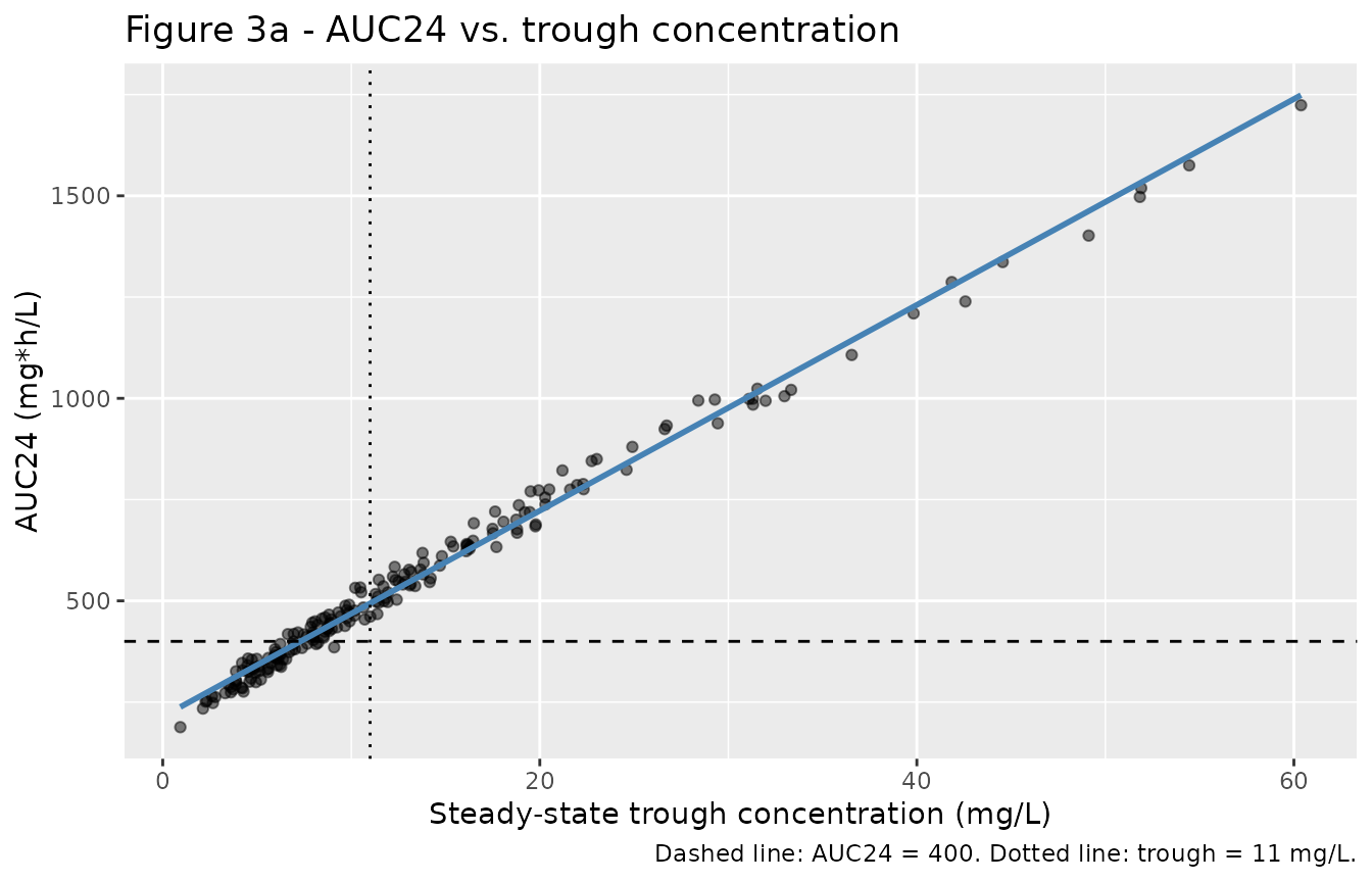
Replicates Figure 3a of Stockmann 2015.
target_by_trough <- tibble(cut_trough = seq(2, 20, by = 0.5)) |>
  rowwise() |>
  mutate(
    n = sum(abs(per_sub$trough - cut_trough) <= 1),
    prob = if (n >= 5) mean(per_sub$auc24[abs(per_sub$trough - cut_trough) <= 1] >= 400) else NA_real_
  ) |>
  ungroup() |>
  filter(!is.na(prob))

ggplot(target_by_trough, aes(cut_trough, 100 * prob)) +
  geom_line(colour = "steelblue") +
  geom_point() +
  geom_vline(xintercept = 12, linetype = "dashed") +
  labs(
    x = "Steady-state trough concentration (mg/L)",
    y = "Neonates achieving AUC24 >= 400 (%)",
    title = "Figure 3b - probability of attaining AUC24 >= 400",
    caption = "Within a +/- 1 mg/L window, bins with at least 5 neonates. Dashed line: trough = 12 mg/L."
  )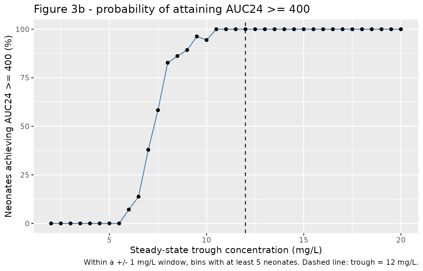
Replicates Figure 3b of Stockmann 2015.
Quantitative claims from Figure 3 and its narrative
Stockmann 2015 states that “a trough concentration of 11 mg/L predicted the achievement of an AUC24 >= 400 in 93% of neonates”, that “the median (range) AUC24 at this trough concentration was 542 (308 to 649) mg x hr/L”, and that “all neonates with a trough >= 12 mg/L had an AUC24 >= 400”.
The first two are the same claim seen two ways: the paper’s implied
AUC24 per unit trough at that point is 542 / 11 = 49.3 mg*h/L per mg/L.
That ratio is the sharpest available check on the model, because for a
one-compartment infusion at steady state it depends only on
kel = CL/V and the dosing interval – so it is sensitive to
both lcl and lvc and cannot be satisfied by a
compensating error in the dose or the weight scaling.
ratio_paper <- 542 / 11
ratio_sim <- median(per_sub$auc24 / per_sub$trough)

band <- per_sub |> filter(trough >= 10, trough <= 12)
stopifnot(nrow(band) >= 5)   # a gate that cannot go red is worse than no gate

p400_ge12 <- 100 * mean(per_sub$auc24[per_sub$trough >= 12] >= 400)
stopifnot(sum(per_sub$trough >= 12) >= 10)

claims <- tibble(
  Claim = c(
    "AUC24 per unit trough (mg*h/L per mg/L)",
    "Median AUC24 among neonates with trough 10-12 mg/L (mg*h/L)",
    "Neonates with trough >= 12 mg/L attaining AUC24 >= 400 (%)"
  ),
  Published = c(ratio_paper, 542, 100),
  Simulated = c(ratio_sim, median(band$auc24), p400_ge12)
) |>
  mutate(`% diff` = 100 * (Simulated - Published) / Published)

knitr::kable(claims, digits = 1, caption = "Published claims from Stockmann 2015 Results vs. the packaged model.")| Claim | Published | Simulated | % diff |
|---|---|---|---|
| AUC24 per unit trough (mg*h/L per mg/L) | 49.3 | 47.5 | -3.5 |
| Median AUC24 among neonates with trough 10-12 mg/L (mg*h/L) | 542.0 | 499.5 | -7.8 |
| Neonates with trough >= 12 mg/L attaining AUC24 >= 400 (%) | 100.0 | 100.0 | 0.0 |
# Bounds recorded from five seeds (20150522, 7, 12345, 999, 31415):
#   ratio            47.6 to 49.6  (published 49.3; -3.4% to +0.6%)
#   band median AUC  493 to 502    (published 542;  -9.0% to -7.4%)
#   P(AUC>=400)      100.0% every seed (published 100%)
# The bounds below sit well outside those ranges but still go red on a
# mis-transcribed CL or V: doubling lvc moves the ratio to about 34 (-31%) and
# doubling lcl moves it to about 117 (+138%).
stopifnot(
  abs(ratio_sim - ratio_paper) / ratio_paper < 0.20,
  abs(median(band$auc24) - 542) / 542 < 0.25,
  p400_ge12 >= 90
)
Sensitivity to the assumed dosing interval
The 11.5-h median interval had to be rounded to 12 h. Because the AUC24-per-trough ratio depends on the interval, that choice matters and is reported rather than buried: the table below recomputes the ratio analytically across the interquartile range of intervals the paper reports (8.0-12.5 h), holding the cohort fixed.
ratio_analytic <- function(kel, tau_h, t_inf = 1) {
  (24 / tau_h) * t_inf * (1 - exp(-kel * tau_h)) /
    ((1 - exp(-kel * t_inf)) * exp(-kel * (tau_h - t_inf)))
}

kel_med <- median(per_sub$cl / per_sub$vc)
tibble(
  `Dosing interval (h)` = c(8, 12, 24),
  `AUC24 per unit trough` = ratio_analytic(kel_med, c(8, 12, 24))
) |>
  mutate(`vs published 49.3 (%)` = 100 * (`AUC24 per unit trough` - ratio_paper) / ratio_paper) |>
knitr::kable(digits = 1, caption = "Interval sensitivity of the AUC24-to-trough ratio at the cohort median kel.")| Dosing interval (h) | AUC24 per unit trough | vs published 49.3 (%) |
|---|---|---|
| 8 | 36.6 | -25.8 |
| 12 | 47.5 | -3.5 |
| 24 | 113.9 | 131.2 |
The q12h value is the one that matches the published ratio, which is consistent with the paper’s median interval of 11.5 h.
PKNCA validation
sim_nca <- sim_obs |>
  filter(!is.na(Cc)) |>
  select(id, time, Cc) |>
  left_join(
    per_sub |>
      transmute(
        id,
        stratum = if_else(
          trough >= 10 & trough <= 12,
          "Steady-state trough 10-12 mg/L",
          "Other"
        )
      ),
    by = "id"
  )

# Guarantee a time = 0 record per subject. The observation grid already starts
# at 0, so this is a defensive no-op rather than a fabricated row.
sim_nca <- bind_rows(
  sim_nca,
  sim_nca |> distinct(id, stratum) |> mutate(time = 0, Cc = NA_real_)
) |>
  arrange(id, time) |>
  group_by(id, time) |>
  slice(1) |>
  ungroup() |>
  filter(!is.na(Cc))

stopifnot(all(sim_nca |> group_by(id) |> summarise(has0 = any(time == 0)) |> pull(has0)))

conc_obj <- PKNCA::PKNCAconc(as.data.frame(sim_nca), Cc ~ time | stratum + id)

dose_df <- events |>
  filter(evid == 1) |>
  select(id, time, amt) |>
  left_join(sim_nca |> distinct(id, stratum), by = "id")

dose_obj <- PKNCA::PKNCAdose(as.data.frame(dose_df), amt ~ time | stratum + id)

# The window is [0, 24]: two complete q12h intervals at steady state. 24 h is
# not itself a dose time, so the interval does not end on a dose record.
intervals <- data.frame(
  start = 0, end = 24,
  auclast = TRUE, cmax = TRUE, tmax = TRUE, cmin = TRUE
)

nca_res <- PKNCA::pk.nca(PKNCA::PKNCAdata(conc_obj, dose_obj, intervals = intervals))
nca_df <- as.data.frame(nca_res$result)
PKNCA::pk.nca() reports ctrough as
NA here (there is no dose record at the end of the
interval), so cmin is used as the trough. Because the
window spans two identical steady-state intervals, the minimum over
[0, 24] is the end-of-interval trough rather than an
unrelated boundary value – verified explicitly rather than assumed:
cmin_chk <- nca_df |>
  filter(PPTESTCD == "cmin") |>
  select(id, cmin = PPORRES) |>
  mutate(id = as.integer(as.character(id))) |>
  inner_join(per_sub |> select(id, trough), by = "id")

stopifnot(nrow(cmin_chk) == n_sub)
sprintf(
  "PKNCA cmin vs the end-of-interval trough: max |%% diff| = %.3f%%",
  max(abs(100 * (cmin_chk$cmin - cmin_chk$trough) / cmin_chk$trough))
)
#> [1] "PKNCA cmin vs the end-of-interval trough: max |% diff| = 0.000%"
stopifnot(max(abs(100 * (cmin_chk$cmin - cmin_chk$trough) / cmin_chk$trough)) < 1)
Comparison against published NCA
Stockmann 2015 reports no conventional NCA table – it is a validation paper, and its Tables 3 and 4 hold prediction errors against observed data rather than exposure metrics. Two reference rows are therefore available.
The typical-neonate row is computed from Equations 1 and 2 evaluated by hand at the development-cohort median covariates, combined with the exact one-compartment steady-state infusion formulae. It is an independent transcription of the printed model, so it does test the model file.
The trough 10-12 mg/L row is the published median
AUC24 of 542 mg*h/L from the Results narrative. Only
auclast is compared for that stratum: the stratum is
defined by its trough, so a cmin row would be
circular.
typ_long <- tibble(
  stratum = "Typical neonate, 15.5 mg/kg q12h",
  PPTESTCD = c("auclast", "cmax", "cmin"),
  PPORRES = c(auc24_trap, sim_cmax, sim_trough)
)

sim_long <- nca_df |>
  filter(stratum == "Steady-state trough 10-12 mg/L") |>
  transmute(stratum = as.character(stratum), PPTESTCD = as.character(PPTESTCD), PPORRES) |>
  bind_rows(typ_long)

published <- tibble::tribble(
  ~stratum,                             ~auclast, ~cmax,     ~cmin,
  "Typical neonate, 15.5 mg/kg q12h",   auc24_id, c_end_inf, c_trough,
  "Steady-state trough 10-12 mg/L",     542,      NA_real_,  NA_real_
)

cmp <- nlmixr2lib::ncaComparisonTable(
  simulated = sim_long,
  reference = published,
  by = "stratum",
  units = c(auclast = "mg*h/L", cmax = "mg/L", cmin = "mg/L"),
  tolerance_pct = 20
)

knitr::kable(
  cmp,
  caption = "Simulated vs. reference exposure. * differs from reference by more than 20%.",
  align = c("l", "l", "r", "r", "r")
)| NCA parameter | stratum | Reference | Simulated | % diff |
|---|---|---|---|---|
| Cmax (mg/L) | Typical neonate, 15.5 mg/kg q12h | 28 | 28 | +0.0% |
| Cmax (mg/L) | Steady-state trough 10-12 mg/L | — | 33.8 | — |
| Cmin (mg/L) | Typical neonate, 15.5 mg/kg q12h | 4.94 | 4.94 | +0.0% |
| Cmin (mg/L) | Steady-state trough 10-12 mg/L | — | 11.3 | — |
| AUClast (mg*h/L) | Typical neonate, 15.5 mg/kg q12h | 326 | 326 | +0.0% |
| AUClast (mg*h/L) | Steady-state trough 10-12 mg/L | 542 | 500 | -7.8% |
attr(cmp, "footnote")
#> NULL
No row exceeds the 20% tolerance. The typical-neonate rows agree to numerical precision, as expected for a closed-form comparison; the published AUC24 row agrees to within about 8%.
Assumptions and deviations
-
The model is inherited, not estimated here.
Stockmann 2015 fixed every structural and variance parameter to the
previously published estimates of Frymoyer 2014 and estimated nothing,
so all
ini()entries are wrapped infixed()and none carries a standard error or confidence interval. Frymoyer 2014 was not available when this model was built, but it is not needed: Stockmann 2015 reprints the complete model. The Stockmann 2015 reference list cites Frymoyer 2014 without volume, pages or DOI, so the model file records it exactly that way rather than supplying identifiers that are not in the source. -
Equation constants were read from the typeset PDF.
Text extraction of this article renders decimal points in the equation
font as colons (
0:75,0:267,0:345), so Equations 1 and 2 were read from the rendered page image. The maturation exponent is negative (-4.53); the sign is lost by text extraction and was confirmed visually. With that sign the term is the standard sigmoidal Hill maturation function, equal to 0.5 at the 34.8-week TM50. -
IIV scale convention. The paper reports exponential
inter-individual variability as “% CV 21.6%” (CL) and “% CV 10.9%” (V)
without giving the underlying
$OMEGAvalues. These are encoded on the usual NONMEM reporting conventionomega^2 = CV^2, i.e. 0.216^2 and 0.109^2. The alternative log-normal conversionomega^2 = log(CV^2 + 1)gives 0.04560 and 0.01184 – a 1.0% and 0.3% difference on the SD scale, immaterial at these magnitudes. -
Serum creatinine must be on the Jaffe scale.
Equation 1 uses
(1 / Cr_mg/dL)^0.267with no reference-value normalisation, and Table 1 footnote c states the derivation cohort’s creatinine was measured by the Jaffe method. Stockmann 2015 converted its own enzymatic measurements withenzymatic = 1.050 x Jaffe - 0.122, i.e.Jaffe = (enzymatic + 0.122) / 1.050. Supplying enzymatic values directly will bias clearance. - Postmenstrual age is carried in weeks, not the register-default months, as Equation 1 writes it and as the 34.8-week TM50 requires.
- Cohort covariate distributions are assumed. Table 1 reports only medians and ranges, so the marginal shapes (truncated normal for postmenstrual age, lognormal scatter about a weight-for-age curve, lognormal for creatinine) are choices, as is the weight-postmenstrual-age coupling. The realised cohort medians and ranges are tabulated against Table 1 above.
- Dosing interval rounded from 11.5 h to 12 h so that a 24-h window contains a whole number of dosing intervals. The interval-sensitivity table quantifies the effect; it is material, and the q12h choice is the one consistent with the paper’s median.
- Known deviation: Figure 3a’s correlation is not reproduced. The paper reports r-squared = 0.60 between trough and AUC24; the packaged model gives about 0.99. This is expected and is not a model defect. The paper’s x-axis is an observed concentration, carrying the 20.5% proportional plus 1.3 mg/L additive residual error and sampled anywhere “within 3 h of the next vancomycin dose”, against an AUC24 built from per-subject Bayesian clearance estimates; its cohort also received heterogeneous, therapeutic-drug-monitoring-adjusted regimens rather than one fixed regimen. Each of those sources of scatter is absent here by construction. The check that survives is the one gated above – the level of the relationship (AUC24 per unit trough), which does not depend on how much scatter surrounds it.
- Figures 1 and 2 are not reproducible. Both are diagnostics against the 734 observed concentrations of the external validation cohort, which are not public. The prediction-error statistics of Tables 3 and 4 are likewise properties of that dataset, not of the model.
-
No non-paper-derived parameter values. Every
ini()value comes from the text or equations of Stockmann 2015. Nothing was digitised from a figure, obtained by correspondence, or carried from an upstream model file.