Levodopa and carbidopa microtablets (Senek 2018)
Source:vignettes/articles/Senek_2018_levodopa_carbidopa.Rmd
Senek_2018_levodopa_carbidopa.RmdModel and source
- Citation: Senek M, Nyholm D, Nielsen EI. Population pharmacokinetics of levodopa/carbidopa microtablets in healthy subjects and Parkinson’s disease patients. Eur J Clin Pharmacol. 2018;74(10):1299-1307. doi:10.1007/s00228-018-2497-2
- Description: Joint population PK model for levodopa and carbidopa after a single dose of dispersible levodopa/carbidopa (4:1) microtablets in healthy adults and in Parkinson’s disease patients with motor fluctuations: levodopa two-compartment and carbidopa one-compartment disposition, each analyte absorbed through two parallel transit-compartment chains (fast and slow) that reproduce double-peak profiles, an estimated pre-dose concentration in patients decaying at the terminal slope, allometric body-weight scaling, a hyperbolic carbidopa-dose inhibition of levodopa CL/F, Hoehn and Yahr stage on both CL/F, age on carbidopa CL/F and levodopa relative bioavailability, and sex on the carbidopa slow-chain mean transit time (Senek 2018)
- Article: https://doi.org/10.1007/s00228-018-2497-2 (open access, CC BY 4.0)
Levodopa/carbidopa 5/1.25 mg microtablets (Flexilev) are dispensed by
an automatic dose dispenser so that a Parkinson’s disease patient can
take small, individually timed doses. Senek 2018 pooled two single-dose
studies, one in healthy volunteers and one in patients with motor
fluctuations, and fitted one joint population PK model for levodopa (LD)
and carbidopa (CD). Both analytes show double-peak profiles, which the
model reproduces with two parallel transit-compartment absorption chains
per analyte: a fraction fa1 of the dose passes through a
fast chain and the rest through a slow one.
Carbidopa inhibits peripheral dopa decarboxylase, and in the model the total carbidopa dose lowers levodopa CL/F hyperbolically: 15% lower at 75 mg than at 50 mg of carbidopa. Levodopa CL/F also falls with Hoehn and Yahr stage (18% from stage 1 to 4), and carbidopa CL/F falls with age (28% from 60 to 80 years).
Population
The model-development data are 36 subjects from two single-centre, open-label, single-dose microtablet studies (Senek 2018 Table 1):
- Study 1: 18 healthy volunteers (9 M / 9 F), age 26.0 +/- 6.2 years (19-46), body weight 71.7 +/- 11.3 kg (59-95). Single dose of 100/25 mg LD/CD, i.e. 20 microtablets dispersed in 100 mL water, sampled to 24 h.
- Study 2: 18 patients with Parkinson’s disease and motor fluctuations (13 M / 5 F; one of 19 enrolled patients was excluded for an extreme triple-peak profile), age 71.4 +/- 6.3 years (61-82), body weight 75.4 +/- 11.0 kg (55-96), Hoehn and Yahr stage 3.2 +/- 0.9 (2-5), 9.6 years since diagnosis. After an overnight washout they took 150% of their individual levodopa-equivalent morning dose, 110/27.5 to 410/102.5 mg (mean 275/68.75 mg), and were sampled to 6 h.
Study 3 (10 healthy volunteers, 4 M / 6 F, age 24.7 +/- 4.3 years, body weight 71.3 +/- 13.7 kg) received 75/18.75 mg followed by five doses of 45/11.25 mg every 2.4 h. It was used only for the external evaluation of the levodopa model (Fig. 2), not for fitting.
The same information is available programmatically via
readModelDb("Senek_2018_levodopa_carbidopa")()$population.
Source trace
Every ini() value carries an in-file comment in
inst/modeldb/specificDrugs/Senek_2018_levodopa_carbidopa.R;
the table collects them. Table 2 values are the NONMEM point estimates
(first two value columns), not the SIR medians.
| Equation / parameter | Value | Source location |
|---|---|---|
| LD two-compartment, CD one-compartment disposition | – | Results, ‘Base model’ |
Two parallel transit chains per analyte; dose split fa1
/ 1 - fa1
|
– | Methods, ‘Base model’; Results, ‘Base model’ |
| Transit compartments: LD 5 (fast) and 6 (slow), CD 3 and 10 | – | Results, ‘Base model’ |
Allometric P = TVP * (WT/70)^E, E = 0.75 for CL/F and
Q/F, 1 for VC/F and VP/F |
– | Methods, ‘Covariate model’, first display equation |
Linear covariate
P = TVP * (1 + coeff * (COV - mean))
|
– | Methods, ‘Covariate model’, second display equation |
Carbidopa-dose interaction
CL/F = TVCL / (1 + CDAMT / INTER)
|
– | Methods, ‘Covariate model’, third display equation |
| Covariate means: sex 0.389, age 48.7 y, HY 1.53 | – | Table 1 footnote |
| Pre-dose concentration decaying at the terminal slope | – | Methods, ‘Base model’ |
lcl (LD CL/F, 0 mg CD, HY 1.53) |
log(1.31) L/min |
Table 2 and footnote dagger |
lvc, lq, lvp
|
log(45.4) L, log(0.667) L/min,
log(44.9) L |
Table 2 |
lmtt1, lmtt2 (LD) |
log(16.1), log(86.2) min |
Table 2 |
logitffo (LD fa1) |
logit(0.749) |
Table 2 (logit scale, footnote double-dagger) |
lfdepot (LD Frel) |
fixed(log(1)) |
Table 2 ‘1 FIX’ |
lc0 (LD pre-dose) |
log(0.120) ug/mL |
Table 2 |
led50 (INTER) |
log(86.7) mg |
Table 2 ‘INTERCL/F-CDAMT’ |
e_dis_pd_hy_cl |
fixed(-0.0616) |
Table 2 ‘CL/F-HY’ |
e_age_fdepot |
fixed(0.00172) |
Table 2 ‘FREL-AGE’ |
lcl_carbidopa, lvc_carbidopa
|
log(1.05) L/min, log(168) L |
Table 2 |
lmtt1_carbidopa, lmtt2_carbidopa
|
log(34.6), log(121) min |
Table 2 |
logitffo_carbidopa (CD fa1) |
logit(0.570) |
Table 2 |
lfdepot_carbidopa |
fixed(log(1)) |
Table 2 ‘1 FIX’ |
lc0_carbidopa |
log(0.0256) ug/mL |
Table 2 |
e_age_cl_carbidopa,
e_dis_pd_hy_cl_carbidopa,
e_sexf_mtt2_carbidopa
|
fixed(-0.0119), fixed(0.0141),
fixed(0.178)
|
Table 2 ‘CL/F-AGE’, ‘CL/F-HY’, ‘MTT2-SEX’ |
e_wt_* allometric exponents |
fixed(0.75) / fixed(1)
|
Methods, ‘Covariate model’ |
| IIV variances | (CV/100)^2 |
Table 2 ‘IIV’ rows (see Assumptions) |
| Residual SDs, healthy / patients | LD 0.150 / 0.0702 and 0.00406 / 0; CD 0.0770 / 0.0386 and 0.00415 / 0.00684 | Table 2 ‘Proportional error’, ‘Additive error’; Results (‘fixed to 0’) |
Reproducing the paper’s derived numbers
The Results and Discussion quote several typical-value consequences
of the covariate model. These are closed-form functions of the
ini() values, so the check is exact: it confirms the
functional forms, the covariate centring and the sex coding in one
pass.
p <- rxode2::rxode(readModelDb("Senek_2018_levodopa_carbidopa"))$theta
#> ℹ parameter labels from comments will be replaced by 'label()'

cl_ld <- function(cd_mg, hy, wt = 70) {
  exp(p[["lcl"]]) * (wt / 70)^0.75 * (1 + p[["e_dis_pd_hy_cl"]] * (hy - 1.53)) *
    exp(p[["led50"]]) / (exp(p[["led50"]]) + cd_mg)
}
cl_cd <- function(age, hy = 1.53, wt = 70) {
  exp(p[["lcl_carbidopa"]]) * (wt / 70)^0.75 *
    (1 + p[["e_age_cl_carbidopa"]] * (age - 48.7)) *
    (1 + p[["e_dis_pd_hy_cl_carbidopa"]] * (hy - 1.53))
}
vc_cd <- function(wt = 70) exp(p[["lvc_carbidopa"]]) * wt / 70
mtt2_cd <- function(sexf) {
  exp(p[["lmtt2_carbidopa"]]) * (1 + p[["e_sexf_mtt2_carbidopa"]] * (sexf - 0.389))
}
frel_ld <- function(age) 1 + p[["e_age_fdepot"]] * (age - 48.7)

derived <- tibble::tribble(
  ~quantity, ~paper, ~model,
  "LD CL/F, 95 mg CD, HY 3, 70 kg (L/h)", 34, 60 * cl_ld(95, 3),
  "LD CL/F reduction, 75 vs 50 mg CD (%)", 15, 100 * (1 - cl_ld(75, 1.53) / cl_ld(50, 1.53)),
  "LD CL/F reduction, HY 1 to 4 (%)", 18, 100 * (1 - cl_ld(0, 4) / cl_ld(0, 1)),
  "LD total volume VC/F + VP/F (L)", 90, exp(p[["lvc"]]) + exp(p[["lvp"]]),
  "CD CL/F, 70 kg, 48.7 y (L/h)", 63, 60 * cl_cd(48.7),
  "CD VC/F, 70 kg (L)", 168, vc_cd(),
  "CD half-life, 70 kg, 48.7 y (min)", 111, log(2) * vc_cd() / cl_cd(48.7),
  "CD half-life, 75.4 kg, 71.4 y (min)", 155, log(2) * vc_cd(75.4) / cl_cd(71.4, wt = 75.4),
  "CD CL/F reduction, age 60 to 80 (%)", 28, 100 * (1 - cl_cd(80) / cl_cd(60)),
  "CD MTT2, women minus men (min)", 22, mtt2_cd(1) - mtt2_cd(0),
  "CD MTT2, women vs men (%)", 19, 100 * (mtt2_cd(1) / mtt2_cd(0) - 1),
  "LD Frel change, age 60 to 80 (%)", 3.4, 100 * (frel_ld(80) / frel_ld(60) - 1)
) |>
  mutate(pct_diff = 100 * (model - paper) / paper)

knitr::kable(
  derived |>
    dplyr::rename(
      "Derived quantity" = quantity,
      "Paper" = paper,
      "Model" = model,
      "% diff" = pct_diff
    ),
  digits = 2,
  caption = "Typical-value quantities quoted in Senek 2018 Results and Discussion, recomputed from the model parameters."
)| Derived quantity | Paper | Model | % diff |
|---|---|---|---|
| LD CL/F, 95 mg CD, HY 3, 70 kg (L/h) | 34.0 | 34.11 | 0.32 |
| LD CL/F reduction, 75 vs 50 mg CD (%) | 15.0 | 15.46 | 3.07 |
| LD CL/F reduction, HY 1 to 4 (%) | 18.0 | 17.90 | -0.58 |
| LD total volume VC/F + VP/F (L) | 90.0 | 90.30 | 0.33 |
| CD CL/F, 70 kg, 48.7 y (L/h) | 63.0 | 63.00 | 0.00 |
| CD VC/F, 70 kg (L) | 168.0 | 168.00 | 0.00 |
| CD half-life, 70 kg, 48.7 y (min) | 111.0 | 110.90 | -0.09 |
| CD half-life, 75.4 kg, 71.4 y (min) | 155.0 | 154.80 | -0.13 |
| CD CL/F reduction, age 60 to 80 (%) | 28.0 | 27.50 | -1.79 |
| CD MTT2, women minus men (min) | 22.0 | 21.54 | -2.10 |
| CD MTT2, women vs men (%) | 19.0 | 19.12 | 0.65 |
| LD Frel change, age 60 to 80 (%) | 3.4 | 3.37 | -0.75 |
# Every quoted number is printed to 2 significant figures, so agreement within
# the rounding of the quote (< 3.5%) is the test.
stopifnot(all(abs(derived$pct_diff) < 3.5))
The carbidopa half-life at the patients’ mean age (155 min) matches only with the patients’ mean body weight (75.4 kg) as well; at 70 kg it would be 152 min. Two further numbers in the paper do not reproduce and are discussed under Assumptions and deviations.
Virtual cohorts
Each simulated cohort has 100 subjects, with covariates drawn to
match Table 1. A dose is given into both dosing compartments of each
analyte: the model’s f() assigns the fraction
fa1 to depot (fast chain) and
1 - fa1 to depot2 (slow chain), so each
analyte needs two dose records of the full amount.
set.seed(2018)
rxode2::rxSetSeed(2018)
n_sub <- 100

rtrunc_norm <- function(n, mean, sd, lo, hi) {
  pmin(pmax(rnorm(n, mean, sd), lo), hi)
}

cohort_study1 <- tibble::tibble(
  id = seq_len(n_sub),
  study = "Study 1 (healthy)",
  WT = rtrunc_norm(n_sub, 71.7, 11.3, 59, 95),
  AGE = rtrunc_norm(n_sub, 26.0, 6.2, 19, 46),
  SEXF = rbinom(n_sub, 1, 9 / 18),
  DIS_PD_HY = 0,
  DIS_HEALTHY = 1,
  dose_ld = 100
)

# Study 2 doses are 150% of the individual morning dose in 5 mg microtablet
# steps (Table 1: 275 +/- 86.3 mg, range 110-410 mg). Hoehn and Yahr stage is
# drawn from {2, 3, 4, 5} with probabilities giving mean 3.2 and SD 0.98.
cohort_study2 <- tibble::tibble(
  id = n_sub + seq_len(n_sub),
  study = "Study 2 (patients)",
  WT = rtrunc_norm(n_sub, 75.4, 11.0, 55, 96),
  AGE = rtrunc_norm(n_sub, 71.4, 6.3, 61, 82),
  SEXF = rbinom(n_sub, 1, 5 / 18),
  DIS_PD_HY = sample(2:5, n_sub, replace = TRUE, prob = c(0.3, 0.3, 0.3, 0.1)),
  DIS_HEALTHY = 0,
  dose_ld = 5 * round(rtrunc_norm(n_sub, 275, 86.3, 110, 410) / 5)
)

cohort_single <- bind_rows(cohort_study1, cohort_study2) |>
  mutate(
    dose_cd = dose_ld / 4,
    # Single dose: the total carbidopa dose of the study is the dose itself.
    DOSE_CARBIDOPA_MG = dose_cd
  )

make_events <- function(cohort, dose_times, dose_ld_fun, obs_times) {
  doses <- cohort |>
    tidyr::crossing(dose_index = seq_along(dose_times)) |>
    mutate(time = dose_times[dose_index], ld = dose_ld_fun(dose_index, dose_ld)) |>
    tidyr::crossing(cmt = c("depot", "depot2", "depot_carbidopa", "depot2_carbidopa")) |>
    mutate(
      amt = ifelse(grepl("carbidopa", cmt), ld / 4, ld),
      evid = 1L,
      dvid = NA_integer_
    ) |>
    select(-dose_index, -ld)
  obs <- cohort |>
    tidyr::crossing(time = obs_times) |>
    mutate(cmt = "central", amt = 0, evid = 0L, dvid = 1L)
  bind_rows(doses, obs) |>
    arrange(id, time, desc(evid)) |>
    select(id, time, amt, cmt, evid, dvid, everything())
}

events_single <- make_events(
  cohort_single,
  dose_times = 0,
  dose_ld_fun = function(i, dose) dose,
  obs_times = c(0, 5, seq(10, 120, by = 10), seq(140, 360, by = 20), seq(420, 720, by = 60))
) |>
  filter(!(study == "Study 2 (patients)" & time > 360))
Simulation
mod <- readModelDb("Senek_2018_levodopa_carbidopa")

sim_single <- rxode2::rxSolve(
  mod,
  events = events_single,
  keep = c("study", "dose_ld", "dose_cd"),
  returnType = "data.frame",
  useLinCmt = FALSE
)
#> ℹ parameter labels from comments will be replaced by 'label()'
Replicate Figure 1
Figure 1 of Senek 2018 is a prediction-corrected VPC of the observed data in each study and analyte. The figure below shows the simulated individual predictions (including between-subject variability, without residual error) as the 10th, 50th and 90th percentiles per nominal time. It is not prediction-corrected, so the Study 2 band also carries the spread of the individual doses.
sim_long <- sim_single |>
  select(id, time, study, Cc, Cc_carbidopa) |>
  pivot_longer(c(Cc, Cc_carbidopa), names_to = "analyte", values_to = "conc") |>
  mutate(analyte = ifelse(analyte == "Cc", "Levodopa", "Carbidopa"))

vpc_single <- sim_long |>
  group_by(study, analyte, time) |>
  summarise(
    p10 = quantile(conc, 0.10),
    p50 = quantile(conc, 0.50),
    p90 = quantile(conc, 0.90),
    .groups = "drop"
  )

ggplot(vpc_single, aes(time, p50)) +
  geom_ribbon(aes(ymin = p10, ymax = p90), fill = "grey80") +
  geom_line() +
  facet_wrap(~ analyte + study, scales = "free") +
  labs(
    x = "Time (min)",
    y = "Plasma concentration (ug/mL)",
    caption = "Replicates Figure 1 of Senek 2018: median and 10th-90th percentile of simulated concentrations."
  )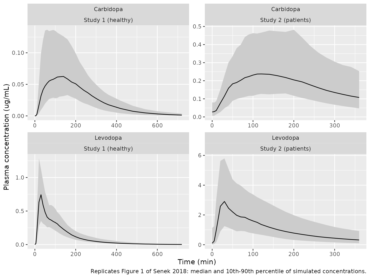
The simulated medians peak near 0.75 ug/mL (levodopa) and 0.06 ug/mL (carbidopa) in healthy volunteers and near 3 ug/mL and 0.24 ug/mL in patients, close to the observed medians of Fig. 1. In the patient panels the curves start from the pre-dose concentration left over from previous treatment.
Replicate Figure 2 (external evaluation, Study 3)
Study 3 gave 75/18.75 mg and then 45/11.25 mg every 2.4 h (144 min), six doses in all. As in the paper, the levodopa CL/F of every Study 3 subject uses the TOTAL carbidopa dose of the regimen, 18.75 + 5 x 11.25 = 75 mg.
cohort_study3 <- tibble::tibble(
  id = 2 * n_sub + seq_len(n_sub),
  study = "Study 3 (healthy, multiple dose)",
  WT = rtrunc_norm(n_sub, 71.3, 13.7, 52, 100),
  AGE = rtrunc_norm(n_sub, 24.7, 4.3, 20, 32),
  SEXF = rbinom(n_sub, 1, 6 / 10),
  DIS_PD_HY = 0,
  DIS_HEALTHY = 1,
  dose_ld = 45,
  DOSE_CARBIDOPA_MG = 18.75 + 5 * 11.25
)
stopifnot(all(cohort_study3$DOSE_CARBIDOPA_MG == 75))

dose_times_3 <- 144 * (0:5)
events_study3 <- make_events(
  cohort_study3,
  dose_times = dose_times_3,
  dose_ld_fun = function(i, dose) ifelse(i == 1, 75, dose),
  obs_times = sort(unique(c(seq(0, 860, by = 10), dose_times_3 + 20, dose_times_3 + 40)))
)

# The six doses deliver 300 mg levodopa and 75 mg carbidopa per subject.
dose_check <- events_study3 |>
  filter(evid == 1, id == min(id)) |>
  group_by(analyte = grepl("carbidopa", cmt)) |>
  summarise(total = sum(amt) / 2)
stopifnot(isTRUE(all.equal(sort(dose_check$total), c(75, 300))))

sim_study3 <- rxode2::rxSolve(
  mod,
  events = events_study3,
  keep = "study",
  returnType = "data.frame",
  useLinCmt = FALSE
)
vpc_study3 <- sim_study3 |>
  group_by(time) |>
  summarise(
    p10 = quantile(Cc, 0.10),
    p50 = quantile(Cc, 0.50),
    p90 = quantile(Cc, 0.90),
    .groups = "drop"
  )

ggplot(vpc_study3, aes(time, p50)) +
  geom_ribbon(aes(ymin = p10, ymax = p90), fill = "grey80") +
  geom_line() +
  labs(
    x = "Time (min)",
    y = "Levodopa plasma concentration (ug/mL)",
    caption = "Replicates Figure 2 of Senek 2018 (Study 3): median and 10th-90th percentile."
  )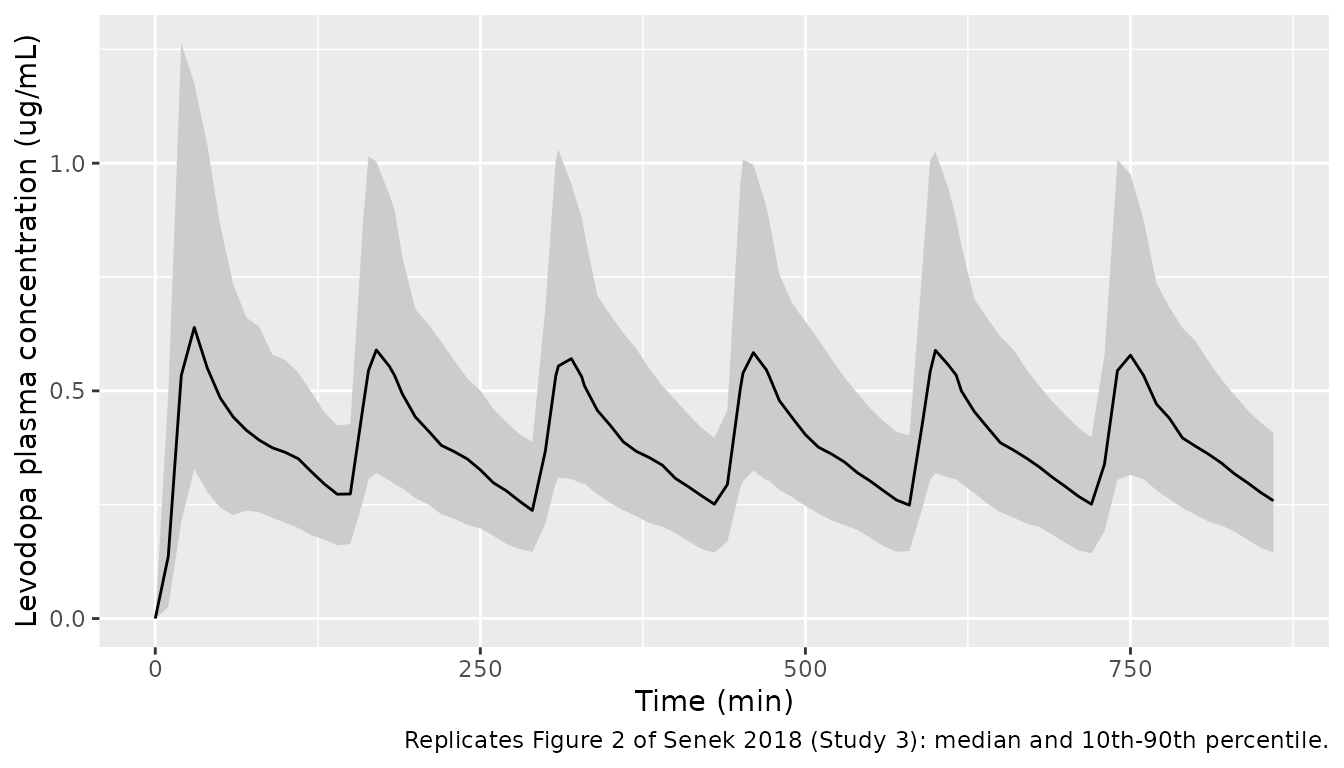
The observed medians in Fig. 2 rise to about 0.6-0.8 ug/mL after each dose and fall to about 0.2 ug/mL before the next. The paper reports that the model over-predicts the first-dose concentrations, which it attributes to the total carbidopa dose being applied from time zero rather than accumulating.
PKNCA validation
Non-compartmental analysis of the simulated single-dose profiles, per study and analyte. The PKNCA dose is the dose of the analyte (one of each pair of dose records, since both carry the full amount).
conc_nca <- sim_long |>
  filter(!is.na(conc)) |>
  rename(treatment = study) |>
  select(id, time, conc, treatment, analyte)

dose_nca <- cohort_single |>
  select(id, treatment = study, Levodopa = dose_ld, Carbidopa = dose_cd) |>
  pivot_longer(c(Levodopa, Carbidopa), names_to = "analyte", values_to = "amt") |>
  mutate(time = 0)

conc_obj <- PKNCA::PKNCAconc(conc_nca, conc ~ time | treatment + analyte + id)
dose_obj <- PKNCA::PKNCAdose(dose_nca, amt ~ time | treatment + analyte + id)

intervals <- data.frame(
  treatment = c("Study 1 (healthy)", "Study 2 (patients)"),
  start = 0,
  end = c(720, 360),
  cmax = TRUE,
  tmax = TRUE,
  auclast = TRUE,
  half.life = TRUE
)

nca_res <- PKNCA::pk.nca(PKNCA::PKNCAdata(conc_obj, dose_obj, intervals = intervals))

nca_summary <- as.data.frame(nca_res) |>
  filter(PPTESTCD %in% c("cmax", "tmax", "auclast", "half.life")) |>
  group_by(treatment, analyte, PPTESTCD) |>
  summarise(median = median(PPORRES, na.rm = TRUE), .groups = "drop") |>
  pivot_wider(names_from = PPTESTCD, values_from = median)

knitr::kable(
  nca_summary |>
    dplyr::rename(
      "Study" = treatment,
      "Analyte" = analyte,
      "Cmax (ug/mL)" = cmax,
      "Tmax (min)" = tmax,
      "AUC0-last (ug*min/mL)" = auclast,
      "t1/2 (min)" = half.life
    ),
  digits = 3,
  caption = "Median simulated NCA parameters per study and analyte."
)| Study | Analyte | AUC0-last (ug*min/mL) | Cmax (ug/mL) | t1/2 (min) | Tmax (min) |
|---|---|---|---|---|---|
| Study 1 (healthy) | Carbidopa | 17.263 | 0.072 | 90.074 | 120 |
| Study 1 (healthy) | Levodopa | 76.997 | 0.827 | 86.975 | 30 |
| Study 2 (patients) | Carbidopa | 61.983 | 0.269 | 148.924 | 120 |
| Study 2 (patients) | Levodopa | 399.172 | 3.250 | 126.174 | 30 |
Comparison against published NCA
Senek 2018 itself reports no NCA table. Its Discussion compares the model’s carbidopa half-life in the patients with the non-compartmental estimate from the original Study 2 publication (Senek 2017), 171 +/- 37 min, and notes that the model value (155 min) is “somewhat lower”. The simulated cohort shows the same shortfall; its median is a little lower again because the simulated patients’ Hoehn and Yahr stages (mean 3.2) raise carbidopa CL/F by about 2% over the reference stage of 1.53 used for the 155 min.
cd_patients <- as.data.frame(nca_res) |>
  filter(treatment == "Study 2 (patients)", analyte == "Carbidopa", PPTESTCD == "half.life")
stopifnot(nrow(cd_patients) == n_sub)

simulated_nca <- cd_patients |>
  transmute(treatment, PPTESTCD, PPORRES)

published <- tibble::tribble(
  ~treatment, ~PPTESTCD, ~PPORRES,
  # Senek 2018 Discussion, citing the NCA of Senek 2017 (reference 6): mean
  # carbidopa half-life 171 +/- 37 min in the Study 2 patients.
  "Study 2 (patients)", "half.life", 171
)

cmp <- nlmixr2lib::ncaComparisonTable(
  simulated = simulated_nca,
  reference = published,
  by = "treatment",
  units = c(half.life = "min"),
  tolerance_pct = 20
)
knitr::kable(
  cmp |>
    dplyr::rename("Study" = treatment),
  caption = "Carbidopa half-life in Parkinson's disease patients: median of the simulated cohort vs the published NCA mean."
)| NCA parameter | Study | Reference | Simulated | % diff |
|---|---|---|---|---|
| t½ (min) | Study 2 (patients) | 171 | 149 | -12.9% |
# The paper's own model value (155 min) is 9% below the NCA and the simulated
# median about 13% below. Dropping the age effect would put it near 113 min
# (-34%), and a volume or clearance mis-transcription moves it further, so a
# 25% band separates those errors from cohort-sampling noise (about 3% SE on a
# median of 100 subjects).
stopifnot(abs(median(cd_patients$PPORRES, na.rm = TRUE) - 171) / 171 < 0.25)
Assumptions and deviations
-
IIV scale. Table 2 prints IIV as “CV%”. It is read
as
100 * sqrt(omega^2)(variance = (CV/100)^2) rather than the log-normalsqrt(exp(omega^2) - 1), for two reasons: the table footnote reports the RSEs “on the approximate standard deviation scale”, which is the PsNsumoconvention of reportingsqrt(omega^2); and the unfixed-coefficient column prints the levodopa pre-dose IIV as1.80where the main column prints180. The two readings agree for the small omegas but not for the pre-dose concentrations: under the log-normal reading the levodopa pre-dose variance would belog(1 + 1.8^2) = 1.44instead of 3.24. -
Distribution of the absorption IIV. Methods says
IIV was “log-normal or normal (absorption-related parameters)”.
fa1is explicitly normal on the logit scale and is encoded that way. MTT1, MTT2 and Frel are encoded log-normal: a normal (TV * (1 + eta)) IIV of 48% on the carbidopa Frel would give negative bioavailabilities in about 2% of subjects, which NONMEM would reject. -
Transit rate constant.
ktr = (n + 1) / MTT, withntransit compartments between the dosing compartment and the central compartment, following Savic 2007, the paper’s reference for the transit model. The paper does not print the formula. -
Pre-dose concentration. Applied to patients only
(
DIS_HEALTHY = 0). The Methods introduce it for the residual levodopa and carbidopa that Study 2 patients carried over despite overnight washout, and the Study 1 and Study 3 panels of Fig. 1 and Fig. 2 start at zero. It is placed at the time of the dose as an initial amount in the central compartment (and, for levodopa, the matching peripheral amount on the slow eigenvector), so that it decays mono-exponentially at the individual terminal slope, as the paper describes. The paper’s observed pre-dose samples were taken up to 1 h before dosing. - Shared residual error not encoded. The paper estimates that 28.5% of the total residual error is shared between levodopa and carbidopa measured in the same sample. nlmixr2 has no construct for a residual correlation across endpoints, so each analyte’s residual error is encoded independently. The marginal residual distribution of each analyte is unchanged; only the correlation between them is lost.
-
Residual error form. The table gives proportional
and additive terms per analyte and population with no further detail;
they are combined as
Var = (prop * C)^2 + add^2. The levodopa additive term in patients was “estimated to a low value … and therefore fixed to 0”. - Unfixed-coefficient variant not shipped. Table 2 also reports a model with re-estimated covariate coefficients and the weaker relationships removed (INTER 119.1 mg, levodopa HY coefficient -0.0967, carbidopa age coefficient -0.0114, no Frel-age, no carbidopa HY, no sex on MTT2). The paper presents it as a sensitivity check of the fixed AALASSO coefficients, so only the final model is encoded.
- Inconsistent levodopa CL/F example. The Results state that INTER = 86.7 mg “results in a LD CL/F estimated to 48.5 L/h with 50 mg CD and 40 L/h with 75 mg CD, for a 70-kg subject”. The model gives 49.9 and 42.1 L/h (at the mean HY of 1.53). The quoted pair implies a 17.5% reduction, while the Abstract quotes 15% for the same comparison, which the model reproduces exactly. The Table 2 parameters and the Abstract are taken as authoritative.
-
Carbidopa HY effect. The Results describe the
carbidopa CL/F change from HY 1 to 4 as “a very modest and clinically
insignificant increase of 0.4%”. The coefficient 0.0141 gives 4.3%
(
(1 + 0.0141 * 2.47) / (1 - 0.0141 * 0.53)), and the same formula reproduces the levodopa HY statement (18%) exactly, so 0.4% is taken to be a dropped digit. - Direction of the age effect on levodopa Frel. The Results call it “a decrease of 3.4% between the age 60 to 80 years”, the Discussion “slightly increased with age (3.4% …)”. The coefficient is positive (0.00172), so Frel increases with age; the model follows the coefficient.
-
Carbidopa dose covariate.
DOSE_CARBIDOPA_MGis the total carbidopa dose over the study period, as in the paper. For a multiple-dose regimen this applies the full inhibition from the first dose. - Virtual cohorts. Table 1 gives means, SDs and ranges only; covariates are drawn from normal distributions truncated to the reported ranges, and the Study 2 Hoehn and Yahr distribution is an assumed discrete distribution with the reported mean.