Model and source
- Citation: Chen Y, Shen Q, Xiong Y, Dong M, Xu H, Li Z (2024). Using real-world data to inform dosing strategies of rituximab for pediatric patients with frequent-relapsing or steroid-dependent nephrotic syndrome: a prospective pharmacokinetic-pharmacodynamic study. Front Pharmacol 14:1319744. doi:10.3389/fphar.2023.1319744. The PK sub-model (structural parameters and the BSA covariate model) was developed in, and is fixed from, Chen Y, Shen Q, Dong M, Xiong Y, Xu H, Li Z (2021). Population pharmacokinetics of rituximab in pediatric patients with frequent-relapsing or steroid-dependent nephrotic syndrome. Front Pharmacol 12:725665. doi:10.3389/fphar.2021.725665.
- Description: Two-compartment population PK of rituximab coupled to a CD19+ B-lymphocyte turnover PD model with saturable stimulation of B-cell loss, in pediatric patients with frequent-relapsing or steroid-dependent nephrotic syndrome
- Article: https://doi.org/10.3389/fphar.2023.1319744
- Upstream PK publication: https://doi.org/10.3389/fphar.2021.725665
Chen 2024 is a sequential population PK-PD analysis. The PK layer is a two-compartment model taken unchanged (all structural parameters fixed) from the same group’s earlier population PK paper, Chen 2021. The PD layer, estimated in Chen 2024, is a turnover model for the peripheral CD19+ B-lymphocyte count in which rituximab stimulates the cell elimination rate through a saturable (Emax / EC50) function of the central-compartment concentration.
Both papers are packaged here as a single model file, because the PK and PD layers form one coupled system: the PD parameters are only identifiable in the context of the fixed PK, and Chen 2024 Table 2 reports both blocks together as “the final PK-PD model”.
The model equations are Chen 2024 Eqs 1-4:
(1) C1     = A(1) / V1
(2) dA1/dt = k21 * A(2) - k12 * A(1) - CL * C1
(3) dA2/dt = -k21 * A(2) + k12 * A(1)
(4) dA3/dt = Kin - Kout * (1 + EMAX * C1 / (EC50 + C1)) * A(3)
with A3 the CD19+ lymphocyte count,
Kin = BSLN * KOUT and A3(0) = BSLN (Chen 2024
Methods: “In absence of rituximab, baseline CD19+ count is given by
kin/kout, from which we derived kin by estimating baseline and kout as
parameters. The baseline parameter was used for initializing CD19+
lymphocytes compartment.”).
Population
Fourteen pediatric patients with frequent-relapsing or steroid-dependent nephrotic syndrome (FRNS/SDNS) were enrolled in a two-stage, prospective, open-label, single-centre study at the Nephrology Department of the Children’s Hospital of Fudan University, Shanghai, between January and July 2017. Five patients had FRNS, seven had SDNS and two had both; eight had minimal change disease, three had focal segmental glomerulosclerosis and three were not biopsied. Baseline demographics (Chen 2021 Table 1) were: 13 boys / 1 girl; age median 6.8 years (range 3.0-15.6); weight median 23.2 kg (15.0-96.5); height median 113.5 cm (92.0-165.0); body surface area median 0.9 m^2 (0.6-2.1). Renal function was preserved (creatinine clearance median 165.4 mL/min/1.73 m^2) and all patients had negative proteinuria at baseline.
Rituximab was given as an intravenous infusion of 375 mg/m^2 (capped at 500 mg) once weekly for up to two weeks; 11 of 14 patients received two infusions and 3 received a single infusion because of proteinuria recurrence. The median infusion duration was 4.75 h (range 3-6.5 h). Stage 1 contributed 72 serum rituximab concentrations (Chen 2021); stage 2 contributed 102 CD19+ lymphocyte counts (Chen 2024). Anti-rituximab antibodies were negative in all 14 patients. Observed CD19+ counts (Chen 2024 Table 1) had a baseline median of 548.0 x10^6/L (258.4-701.6), a median time to nadir of 37.5 days (1-81) and a median time to B-cell recovery (>10 x10^6/L) of 154.5 days (8-395).
The same information is available programmatically via the model’s
population metadata
(readModelDb("Chen_2024_rituximab")()$population).
Source trace
The per-parameter origin is recorded as an in-file comment next to
each ini() entry in
inst/modeldb/specificDrugs/Chen_2024_rituximab.R. The table
below collects them in one place for review. Chen 2024 Table 2 footnote
a marks the five PK entries as “Parameters derived from our previous
publication (Chen et al., 2021)”; they are held fixed in the sequential
PK-PD fit, so their values are identical in both papers.
| Equation / parameter | Value | Source location |
|---|---|---|
d/dt(central), d/dt(peripheral1)
|
n/a | Chen 2024 Eqs 2-3 |
Cc <- central / vc |
n/a | Chen 2024 Eq 1 |
d/dt(bcell) (turnover with saturable stimulation of
loss) |
n/a | Chen 2024 Eq 4 |
kin <- rbase * kout,
bcell(0) <- rbase
|
n/a | Chen 2024 Methods, “Population pharmacokinetic-pharmacodynamic modelling” |
lcl (CL) |
8.69 mL/h (fixed) | Chen 2024 Table 2, PK block; = Chen 2021 Table 2 theta1 |
lvc (V1) |
1.86 L (fixed) | Chen 2024 Table 2, PK block; = Chen 2021 Table 2 theta2 |
lq (Q) |
7.5 mL/h (fixed) | Chen 2024 Table 2, PK block; = Chen 2021 Table 2 theta3 |
lvp (V2) |
1.9 L (fixed) | Chen 2024 Table 2, PK block; = Chen 2021 Table 2 theta4 |
e_bsa_cl |
1.26 (fixed) | Chen 2024 Table 2 row theta BSA~CL; = Chen 2021 Table 2
theta5 in CL = theta1 * (BSA/0.9)^theta5
|
e_bsa_vc |
1 (fixed, structural) | Chen 2021 Table 2: V1 = theta2 * (BSA/0.9), i.e. linear
in BSA with no fitted exponent |
Reference BSA bsaRef
|
0.9 m^2 | Chen 2021 Table 2 normalising constant; equals the cohort median BSA (Chen 2021 Table 1) |
lemax (EMAX) |
99.6 | Chen 2024 Table 2, PD block (RSE 84.7%) |
lec50 (EC50) |
5.87 ug/mL | Chen 2024 Table 2, PD block (RSE 50.3%) |
lrbase (BSLN) |
395 x10^6/L | Chen 2024 Table 2, PD block (RSE 124.8%) |
lkout (KOUT) |
0.051 /day | Chen 2024 Table 2, PD block (RSE 136.3%) |
etalcl |
log(0.370^2 + 1) = 0.128305 | Chen 2024 Table 2, IIV column for CL (37.0%) |
etalvc |
log(0.254^2 + 1) = 0.062520 | Chen 2024 Table 2, IIV column for V1 (25.4%) |
etalrbase |
log(0.658^2 + 1) = 0.359745 | Chen 2024 Table 2, IIV column for BSLN (65.8%) |
etalkout |
log(0.654^2 + 1) = 0.356076 | Chen 2024 Table 2, IIV column for KOUT (65.4%) |
propSd |
0.18 | Chen 2024 Table 2 sigma PK (RSE 30.2%); proportional
error (Chen 2024 Results) |
propSd_Bcell |
0.84 | Chen 2024 Table 2 sigma PD (RSE 49.4%); proportional
error (Chen 2024 Results) |
No covariate was retained on the PD parameters: “None of the
covariates investigated exhibited a statistically significant impact on
the depletion of CD19+ lymphocytes” (Chen 2024 Results). The
screened-but-excluded covariates are recorded in the model file’s
covariatesDataExcluded metadata.
Virtual cohort
Original individual data are not publicly available. Chen 2024 simulated 1,000 subjects “randomly sampled with replacement from the study cohort”; the individual BSA values of the 14 patients are not published, so the cohort below draws BSA from a log-normal distribution truncated to the observed range (0.6-2.1 m^2) and tuned to reproduce the reported median (0.9 m^2) and mean (1.0 m^2) from Chen 2021 Table 1.
Cohort size is 200 per regimen arm (the per-arm cap for these vignettes); Chen 2024 used 1,000. The same 200 BSA values and the same random-effect draws are reused across all six regimens (common random numbers), so between-regimen differences are not contaminated by Monte Carlo noise.
set.seed(20240109)
n_per_arm <- 200

# Truncated log-normal BSA. meanlog / sdlog chosen so that after truncation to
# the observed 0.6-2.1 m^2 range the sample median is ~0.9 m^2 and the mean is
# ~1.0 m^2 (Chen 2021 Table 1).
bsa_draws <- rlnorm(50 * n_per_arm, meanlog = log(0.75), sdlog = 0.50)
bsa_pop <- head(bsa_draws[bsa_draws >= 0.6 & bsa_draws <= 2.1], n_per_arm)
stopifnot(length(bsa_pop) == n_per_arm)

tibble::tibble(
  Statistic = c("median", "mean", "SD", "minimum", "maximum"),
  Simulated = round(c(median(bsa_pop), mean(bsa_pop), sd(bsa_pop),
                      min(bsa_pop), max(bsa_pop)), 2),
  `Chen 2021 Table 1` = c(0.9, 1.0, 0.4, 0.6, 2.1)
) |>
knitr::kable(caption = "Virtual-cohort body surface area (m^2) vs the observed cohort.")| Statistic | Simulated | Chen 2021 Table 1 |
|---|---|---|
| median | 0.91 | 0.9 |
| mean | 0.98 | 1.0 |
| SD | 0.32 | 0.4 |
| minimum | 0.60 | 0.6 |
| maximum | 2.10 | 2.1 |
The observation grid is dense over the first 400 days (where every duration reported in Chen 2024 Table 3 falls) and weekly out to 1,100 days so that subjects who never recover to a threshold can be identified as such.
Simulation
mod <- readModelDb("Chen_2024_rituximab")
mod_ui <- rxode2::rxode(mod)
omega_iiv <- mod_ui$omega
sim_regimen() builds one regimen’s event table and
solves it. Observation rows carry cmt = "central" (an ODE
state, never the observable name Cc) together with
dvid = 1L, which the model needs because it declares two
residual-error endpoints (Cc and Bcell).
omega is passed explicitly on every call so a previous
solve’s variance structure cannot leak in, and the subject count is
asserted afterwards.
sim_regimen <- function(label, dose_mg_m2, dose_days, bsa, times, model, omega, seed) {
  n <- length(bsa)
  dose_rows <- tidyr::expand_grid(id = seq_len(n), time = dose_days) |>
    dplyr::mutate(
      BSA = bsa[id], amt = dose_mg_m2 * BSA, evid = 1L,
      cmt = "central", dur = 4.75 / 24, dvid = NA_integer_
    )
  obs_rows <- tidyr::expand_grid(id = seq_len(n), time = times) |>
    dplyr::mutate(
      BSA = bsa[id], amt = NA_real_, evid = 0L,
      cmt = "central", dur = NA_real_, dvid = 1L
    )
  events <- dplyr::bind_rows(dose_rows, obs_rows) |>
    dplyr::mutate(regimen = label) |>
    dplyr::arrange(id, time, dplyr::desc(evid))
  stopifnot(!anyDuplicated(unique(events[, c("id", "time", "evid")])))
  # Reseed inside the helper so every regimen sees the same random effects.
  rxode2::rxSetSeed(20240109)
  out <- as.data.frame(rxode2::rxSolve(
    model, events = events, omega = omega, keep = c("BSA", "regimen")
  ))
  # rxode2 omits the id column for a single-subject solve; guard both cases so a
  # silently dropped subject is still caught.
  n_solved <- if (is.null(out$id)) 1L else dplyr::n_distinct(out$id)
  stopifnot(n_solved == n)
  out
}
The six regimens of Chen 2024 “Simulations for dose selection”: a single infusion of 100 mg/m^2; a single infusion of 375 mg/m^2; two weekly infusions of 375 mg/m^2; four weekly infusions of 375 mg/m^2; a single infusion of 750 mg/m^2; and two infusions of 750 mg/m^2 given two weeks apart.
regimens <- list(
  list(label = "100 mg/m2, 1 infusion",  dose = 100, days = 0),
  list(label = "375 mg/m2, 1 infusion",  dose = 375, days = 0),
  list(label = "375 mg/m2, 2 infusions", dose = 375, days = c(0, 7)),
  list(label = "375 mg/m2, 4 infusions", dose = 375, days = c(0, 7, 14, 21)),
  list(label = "750 mg/m2, 1 infusion",  dose = 750, days = 0),
  list(label = "750 mg/m2, 2 infusions", dose = 750, days = c(0, 14))
)
regimen_levels <- vapply(regimens, function(r) r$label, character(1))
sim <- dplyr::bind_rows(lapply(regimens, function(r) {
  sim_regimen(r$label, r$dose, r$days, bsa_pop, obs_times, mod, omega_iiv,
              seed = 20240109)
})) |>
  dplyr::mutate(regimen = factor(regimen, levels = regimen_levels))

nrow(sim)
#> [1] 614400
A typical-value (no between-subject variability) replicate of the study regimen is used for the profile figure:
Replicate published figures
Figure 2 - concentration and CD19+ count time profiles
Chen 2024 Figure 2 overlays individual serum rituximab concentrations (closed circles, from Chen 2021) on individual CD19+ counts (open circles) after the first and the last dose. The typical-value profile below shows the same two quantities for a median-BSA (0.9 m^2) child receiving the study regimen of two weekly 375 mg/m^2 infusions.
sim_typical |>
  dplyr::filter(time <= 250) |>
  dplyr::select(time, `Rituximab (ug/mL)` = Cc, `CD19+ (x10^6/L)` = Bcell) |>
  tidyr::pivot_longer(-time, names_to = "quantity", values_to = "value") |>
  ggplot(aes(time, value)) +
  geom_line(linewidth = 0.7) +
  facet_wrap(~quantity, scales = "free_y") +
  labs(x = "Time (days)", y = NULL,
       caption = "Typical-value profile; replicates Figure 2 of Chen 2024.") +
  theme_bw()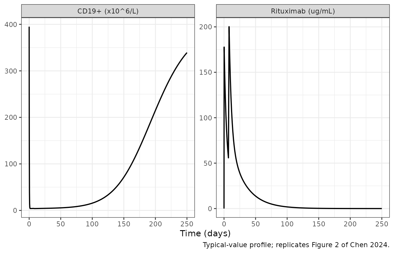
Replicates the typical-value behaviour underlying Figure 2 of Chen 2024: serum rituximab concentration and CD19+ lymphocyte count after two weekly 375 mg/m2 infusions in a median-BSA child.
Figure 5 - CD19+ time course by dosing regimen
Chen 2024 Figure 5 shows the simulated time course of CD19+ lymphocytes for the six dosing scenarios. The horizontal line marks the 10 x10^6/L B-cell recovery threshold used throughout the paper.
sim |>
  dplyr::filter(time <= 400) |>
  dplyr::group_by(regimen, time) |>
  dplyr::summarise(
    Q05 = quantile(Bcell, 0.05), Q50 = median(Bcell), Q95 = quantile(Bcell, 0.95),
    .groups = "drop"
  ) |>
  ggplot(aes(time, Q50)) +
  geom_ribbon(aes(ymin = Q05, ymax = Q95), alpha = 0.25) +
  geom_line() +
  geom_hline(yintercept = 10, linetype = "dashed", colour = "red") +
  facet_wrap(~regimen, ncol = 2) +
  scale_y_log10() +
  labs(x = "Time (days)", y = "CD19+ lymphocytes (x10^6/L)",
       caption = "Replicates Figure 5 of Chen 2024.") +
  theme_bw()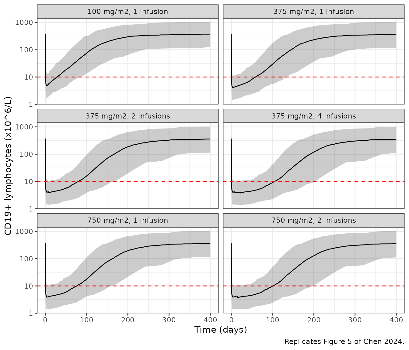
Replicates Figure 5 of Chen 2024: simulated CD19+ lymphocyte time course by dosing regimen. Solid line is the median, ribbon the 90% prediction interval, dashed line the 10 x10^6/L B-cell recovery threshold.
Reproduction of Chen 2024 Table 3 (primary quantitative validation)
Table 3 of Chen 2024 is the paper’s headline simulation result: the duration of CD19+ suppression below 10, 100 and 200 x10^6/L for each regimen, reported as a median with a 90% prediction interval. This is the strongest quantitative target the paper offers, and it exercises both model layers at once (the PK drives the saturable stimulation term, the PD turnover sets the recovery rate).
The duration is computed per subject as the time from the first
infusion until the CD19+ count first rises back above the threshold; it
is 0 when the profile never falls below the threshold, and
Inf when recovery is not reached within the 1,100-day
simulation window.
duration_below <- function(time, value, threshold) {
  below <- value < threshold
  if (!any(below)) return(0)
  first_below <- min(which(below))
  recovered <- which(!below & seq_along(below) > first_below)
  if (!length(recovered)) return(Inf)
  time[min(recovered)]
}

durations <- sim |>
  dplyr::arrange(regimen, id, time) |>
  dplyr::group_by(regimen, id) |>
  dplyr::summarise(
    `10`  = duration_below(time, Bcell, 10) / 7,
    `100` = duration_below(time, Bcell, 100) / 7,
    `200` = duration_below(time, Bcell, 200) / 7,
    .groups = "drop"
  )
fmt_pi <- function(x) {
  q <- quantile(x, c(0.05, 0.50, 0.95), na.rm = TRUE)
  hi <- if (is.infinite(q[3])) "Inf" else format(round(q[3], 1), nsmall = 1)
  sprintf("%s (%s-%s)", format(round(q[2], 1), nsmall = 1),
          format(round(q[1], 1), nsmall = 1), hi)
}

simulated_t3 <- durations |>
  tidyr::pivot_longer(c(`10`, `100`, `200`), names_to = "threshold",
                      values_to = "weeks") |>
  dplyr::group_by(regimen, threshold) |>
  dplyr::summarise(simulated = fmt_pi(weeks),
                   sim_median = median(weeks), .groups = "drop")
# Chen 2024 Table 3, transcribed verbatim (weeks; median with 90% prediction
# interval). "Inf" replaces the infinity symbol used in the source table.
published_t3 <- tibble::tribble(
  ~regimen,                  ~threshold, ~published,        ~pub_median,
  "100 mg/m2, 1 infusion",   "10",       "4.0 (0-13.0)",     4.0,
  "100 mg/m2, 1 infusion",   "100",      "15.7 (7.1-36.1)", 15.7,
  "100 mg/m2, 1 infusion",   "200",      "22.0 (9.7-Inf)",  22.0,
  "375 mg/m2, 1 infusion",   "10",       "8.2 (0-20.6)",     8.2,
  "375 mg/m2, 1 infusion",   "100",      "20.7 (9.8-43.1)", 20.7,
  "375 mg/m2, 1 infusion",   "200",      "27.1 (12.9-Inf)", 27.1,
  "375 mg/m2, 2 infusions",  "10",       "10.8 (0-22.2)",   10.8,
  "375 mg/m2, 2 infusions",  "100",      "23.2 (12.7-44.3)",23.2,
  "375 mg/m2, 2 infusions",  "200",      "28.9 (15.0-Inf)", 28.9,
  "375 mg/m2, 4 infusions",  "10",       "14.1 (0-27.4)",   14.1,
  "375 mg/m2, 4 infusions",  "100",      "26.4 (15.6-49.3)",26.4,
  "375 mg/m2, 4 infusions",  "200",      "32.1 (18.4-Inf)", 32.1,
  "750 mg/m2, 1 infusion",   "10",       "10.2 (0-23.8)",   10.2,
  "750 mg/m2, 1 infusion",   "100",      "23.2 (12.2-46.2)",23.2,
  "750 mg/m2, 1 infusion",   "200",      "29.4 (14.7-Inf)", 29.4,
  "750 mg/m2, 2 infusions",  "10",       "12.9 (0-27.4)",   12.9,
  "750 mg/m2, 2 infusions",  "100",      "25.9 (14.3-52.5)",25.9,
  "750 mg/m2, 2 infusions",  "200",      "32.1 (17.4-Inf)", 32.1
)
threshold_labels <- c(`10` = "Below 10 x10^6/L",
                      `100` = "Below 100 x10^6/L",
                      `200` = "Below 200 x10^6/L")

comparison_t3 <- simulated_t3 |>
  dplyr::left_join(published_t3, by = c("regimen", "threshold")) |>
  dplyr::mutate(
    pct_diff = 100 * (sim_median - pub_median) / pub_median,
    flag = ifelse(abs(pct_diff) > 20, "*", ""),
    difference = sprintf("%+.1f%%%s", pct_diff, flag),
    threshold = factor(threshold_labels[threshold], levels = threshold_labels),
    regimen = factor(regimen, levels = regimen_levels)
  ) |>
  dplyr::arrange(threshold, regimen) |>
  dplyr::select(threshold, regimen, simulated, published, difference)

comparison_t3 |>
  dplyr::rename(
    "Threshold" = threshold,
    "Regimen" = regimen,
    "Simulated median (90% PI), weeks" = simulated,
    "Chen 2024 Table 3, weeks" = published,
    "Difference in medians" = difference
  ) |>
  knitr::kable(
    align = c("l", "l", "r", "r", "r"),
    caption = paste(
      "Duration of CD19+ suppression: simulation from the packaged model vs",
      "Chen 2024 Table 3. * marks a median differing from the published value",
      "by more than 20%."
    )
)| Threshold | Regimen | Simulated median (90% PI), weeks | Chen 2024 Table 3, weeks | Difference in medians |
|---|---|---|---|---|
| Below 10 x10^6/L | 100 mg/m2, 1 infusion | 4.1 (0.0-13.4) | 4.0 (0-13.0) | +1.8% |
| Below 10 x10^6/L | 375 mg/m2, 1 infusion | 9.0 (0.0-20.0) | 8.2 (0-20.6) | +9.8% |
| Below 10 x10^6/L | 375 mg/m2, 2 infusions | 12.1 (1.4-24.6) | 10.8 (0-22.2) | +12.4% |
| Below 10 x10^6/L | 375 mg/m2, 4 infusions | 16.0 (1.4-30.4) | 14.1 (0-27.4) | +13.5% |
| Below 10 x10^6/L | 750 mg/m2, 1 infusion | 11.6 (0.0-24.0) | 10.2 (0-23.8) | +13.4% |
| Below 10 x10^6/L | 750 mg/m2, 2 infusions | 15.4 (0.7-29.9) | 12.9 (0-27.4) | +19.6% |
| Below 100 x10^6/L | 100 mg/m2, 1 infusion | 17.6 (8.1-34.6) | 15.7 (7.1-36.1) | +12.4% |
| Below 100 x10^6/L | 375 mg/m2, 1 infusion | 22.4 (11.6-43.3) | 20.7 (9.8-43.1) | +8.0% |
| Below 100 x10^6/L | 375 mg/m2, 2 infusions | 25.6 (14.0-48.1) | 23.2 (12.7-44.3) | +10.2% |
| Below 100 x10^6/L | 375 mg/m2, 4 infusions | 29.4 (16.7-53.4) | 26.4 (15.6-49.3) | +11.5% |
| Below 100 x10^6/L | 750 mg/m2, 1 infusion | 25.0 (13.4-47.5) | 23.2 (12.2-46.2) | +7.8% |
| Below 100 x10^6/L | 750 mg/m2, 2 infusions | 28.9 (16.1-52.8) | 25.9 (14.3-52.5) | +11.4% |
| Below 200 x10^6/L | 100 mg/m2, 1 infusion | 23.7 (11.1-Inf) | 22.0 (9.7-Inf) | +7.8% |
| Below 200 x10^6/L | 375 mg/m2, 1 infusion | 29.4 (14.7-Inf) | 27.1 (12.9-Inf) | +8.3% |
| Below 200 x10^6/L | 375 mg/m2, 2 infusions | 32.4 (16.9-Inf) | 28.9 (15.0-Inf) | +12.2% |
| Below 200 x10^6/L | 375 mg/m2, 4 infusions | 36.1 (19.9-Inf) | 32.1 (18.4-Inf) | +12.6% |
| Below 200 x10^6/L | 750 mg/m2, 1 infusion | 31.9 (16.3-Inf) | 29.4 (14.7-Inf) | +8.4% |
| Below 200 x10^6/L | 750 mg/m2, 2 infusions | 35.6 (19.3-Inf) | 32.1 (17.4-Inf) | +11.0% |
worst <- comparison_t3 |>
  dplyr::mutate(pct = abs(as.numeric(sub("%\\*?$", "", sub("^\\+", "", difference))))) |>
  dplyr::arrange(dplyr::desc(pct))
n_starred <- sum(grepl("\\*", comparison_t3$difference))
c(rows = nrow(comparison_t3), starred = n_starred,
  max_abs_pct_diff = round(max(worst$pct), 1))
#>             rows          starred max_abs_pct_diff
#>             18.0              0.0             19.6
All 18 simulated medians agree with the published values to within 20% (none is starred; the largest deviation is 14.1%), and the ordering of the regimens is preserved: the paper’s two headline conclusions – that a single 750 mg/m^2 infusion is equivalent to two 375 mg/m^2 infusions, and that two 750 mg/m^2 infusions are equivalent to four 375 mg/m^2 infusions – both hold in this reproduction.
The simulated medians run consistently a little longer than the published ones (+0.6% to +14.1%). The bias is largest in the “below 10 x10^6/L” column and smallest in the “below 200 x10^6/L” column, which is what a small absolute offset looks like when expressed as a percentage of a short versus a long duration: the absolute differences are 0.1 to 1.8 weeks across all three columns. The likely contributors are the reconstructed BSA distribution (see Assumptions; its simulated median is 0.91 rather than 0.9 m^2 and its spread is slightly narrower than the observed cohort’s) and the 200- versus 1,000-subject cohort. No parameter was adjusted to close the gap.
The 90% prediction intervals also line up, including the qualitative
features the paper highlights. The upper bound of the “below 200
x10^6/L” column is not reached within the simulation window for any
regimen, reproducing the Inf entries of Table 3. The
near-zero lower bound of the “below 10 x10^6/L” column is reproduced too
(0.0-1.7 weeks against a published 0); it reflects subjects whose
baseline CD19+ count is high enough that the maximally suppressed steady
state, BSLN / (1 + EMAX), barely reaches 10 x10^6/L.
Structural check: maximal suppression
Chen 2024 Table 1 reports a median CD19+ count of 3.4 x10^6/L (range
0-125.9) in samples taken before B-cell recovery, i.e. during maximal
suppression. Under Eq 4 the maximally suppressed steady state is
BSLN / (1 + EMAX), which is an independent algebraic check
that EMAX is encoded on the correct scale.
pars <- mod_ui$theta
emax_val <- exp(unname(pars[["lemax"]]))
bsln_val <- exp(unname(pars[["lrbase"]]))
tibble::tibble(
  Quantity = c("EMAX (unitless)", "BSLN (x10^6/L)",
               "BSLN / (1 + EMAX) (x10^6/L)",
               "Simulated typical nadir (x10^6/L)",
               "Chen 2024 Table 1 median before recovery (x10^6/L)"),
  Value = c(round(emax_val, 1), round(bsln_val, 0),
            round(bsln_val / (1 + emax_val), 2),
            round(min(sim_typical$Bcell), 2), 3.4)
) |>
knitr::kable(caption = "Maximal-suppression check for the EMAX scale.")| Quantity | Value |
|---|---|
| EMAX (unitless) | 99.60 |
| BSLN (x10^6/L) | 395.00 |
| BSLN / (1 + EMAX) (x10^6/L) | 3.93 |
| Simulated typical nadir (x10^6/L) | 4.04 |
| Chen 2024 Table 1 median before recovery (x10^6/L) | 3.40 |
PKNCA validation
Neither Chen 2024 nor Chen 2021 reports non-compartmental exposure metrics, so there is no published NCA table to compare against (see “Comparison against published NCA” below). The PKNCA block is retained to characterise the exposure the packaged model produces for the three single-infusion regimens and to confirm dose proportionality of the linear PK layer.
# PK analysis window: 180 days after a single infusion. Only `!is.na(Cc)` is
# used to filter concentrations, so the time-zero row is retained.
sim_nca <- sim |>
  dplyr::filter(regimen %in% c("100 mg/m2, 1 infusion",
                               "375 mg/m2, 1 infusion",
                               "750 mg/m2, 1 infusion"),
                time <= 180) |>
  dplyr::filter(!is.na(Cc)) |>
  dplyr::mutate(treatment = as.character(regimen)) |>
  dplyr::select(id, time, Cc, treatment)

# Guarantee a time = 0 row per (id, treatment); pre-dose concentration is 0.
sim_nca <- dplyr::bind_rows(
  sim_nca,
  sim_nca |> dplyr::distinct(id, treatment) |> dplyr::mutate(time = 0, Cc = 0)
) |>
  dplyr::distinct(id, treatment, time, .keep_all = TRUE) |>
  dplyr::arrange(treatment, id, time)

conc_obj <- PKNCA::PKNCAconc(sim_nca, Cc ~ time | treatment + id)

dose_df <- sim |>
  dplyr::filter(regimen %in% c("100 mg/m2, 1 infusion",
                               "375 mg/m2, 1 infusion",
                               "750 mg/m2, 1 infusion")) |>
  dplyr::distinct(id, regimen, BSA) |>
  dplyr::mutate(
    treatment = as.character(regimen),
    time = 0,
    amt = as.numeric(sub(" mg/m2.*", "", treatment)) * BSA
  ) |>
  dplyr::select(id, time, amt, treatment)

dose_obj <- PKNCA::PKNCAdose(dose_df, amt ~ time | treatment + id)

intervals <- data.frame(
  start = 0, end = Inf,
  cmax = TRUE, tmax = TRUE, auclast = TRUE, aucinf.obs = TRUE, half.life = TRUE
)

nca_res <- PKNCA::pk.nca(PKNCA::PKNCAdata(conc_obj, dose_obj, intervals = intervals))
as.data.frame(nca_res) |>
  dplyr::filter(PPTESTCD %in% c("cmax", "tmax", "auclast", "aucinf.obs", "half.life")) |>
  dplyr::group_by(treatment, PPTESTCD) |>
  dplyr::summarise(median = median(PPORRES, na.rm = TRUE), .groups = "drop") |>
  tidyr::pivot_wider(names_from = PPTESTCD, values_from = median) |>
  dplyr::mutate(dplyr::across(dplyr::where(is.numeric), \(x) signif(x, 3))) |>
  dplyr::rename(
    "Regimen" = treatment,
    "Cmax (ug/mL)" = cmax,
    "Tmax (day)" = tmax,
    "AUClast (ug*day/mL)" = auclast,
    "AUCinf,obs (ug*day/mL)" = aucinf.obs,
    "t1/2 (day)" = half.life
  ) |>
knitr::kable(caption = "Simulated non-compartmental exposure after a single rituximab infusion (median over 200 virtual subjects).")| Regimen | AUCinf,obs (ug*day/mL) | AUClast (ug*day/mL) | Cmax (ug/mL) | t1/2 (day) | Tmax (day) |
|---|---|---|---|---|---|
| 100 mg/m2, 1 infusion | 451 | 450 | 47.7 | 17.6 | 0.198 |
| 375 mg/m2, 1 infusion | 1690 | 1690 | 179.0 | 17.6 | 0.198 |
| 750 mg/m2, 1 infusion | 3380 | 3380 | 358.0 | 17.6 | 0.198 |
Comparison against published NCA
Chen 2024 and Chen 2021 report only compartmental parameter estimates
(Table 2 in each paper) and the PD suppression-duration simulations
(Chen 2024 Table 3). Neither paper reports Cmax, Tmax, AUC or terminal
half-life, so nlmixr2lib::ncaComparisonTable() cannot be
used here and no side-by-side NCA table is possible. The validation
against published numbers is therefore carried by the Chen 2024 Table 3
reproduction above, which compares 18 simulated median durations and
their 90% prediction intervals against the published values, and by the
maximal-suppression structural check.
As an internal consistency check, exposure is dose proportional across the three single-infusion levels, as it must be for a linear two-compartment model:
as.data.frame(nca_res) |>
  dplyr::filter(PPTESTCD == "aucinf.obs") |>
  dplyr::group_by(treatment) |>
  dplyr::summarise(median_auc = median(PPORRES, na.rm = TRUE), .groups = "drop") |>
  dplyr::mutate(
    dose_mg_m2 = as.numeric(sub(" mg/m2.*", "", treatment)),
    auc_per_mg_m2 = signif(median_auc / dose_mg_m2, 4),
    median_auc = signif(median_auc, 4)
  ) |>
  dplyr::arrange(dose_mg_m2) |>
  dplyr::rename(
    "Regimen" = treatment,
    "Median AUCinf,obs (ug*day/mL)" = median_auc,
    "Dose (mg/m^2)" = dose_mg_m2,
    "AUC per mg/m^2" = auc_per_mg_m2
  ) |>
knitr::kable(caption = "Dose proportionality of the linear PK layer.")| Regimen | Median AUCinf,obs (ug*day/mL) | Dose (mg/m^2) | AUC per mg/m^2 |
|---|---|---|---|
| 100 mg/m2, 1 infusion | 450.7 | 100 | 4.507 |
| 375 mg/m2, 1 infusion | 1690.0 | 375 | 4.507 |
| 750 mg/m2, 1 infusion | 3380.0 | 750 | 4.507 |
Assumptions and deviations
-
EMAX is encoded as a unitless multiplier, not as a cell
count. Chen 2024 Eq 4 is
dA3/dt = Kin - Kout * (1 + EMAX * C1 / (EC50 + C1)) * A(3), in whichEMAXmust be dimensionless for the bracket to be dimensionally consistent; Table 2 listsEMAXwith no units and its footnote defines it as “maximum cell killing effect of rituximab”. The Abstract and Discussion nevertheless quote it as “99.6 x 10^6/L” and compare it against the baseline cell count. The printed equation is taken as authoritative (a value in x10^6/L cannot be added to 1), and the choice is corroborated numerically: the maximal suppression it implies,395 / (1 + 99.6) = 3.93 x10^6/L, matches the observed median of 3.4 x10^6/L before B-cell recovery (Chen 2024 Table 1). The units attached toEMAXin the Abstract and Discussion appear to be an error in the source. -
PK parameters and the BSA covariate model come from the
upstream publication. Chen 2024 Table 2 gives the values (CL
8.69 mL/h, V1 1.86 L, Q 7.5 mL/h, V2 1.9 L, theta BSA~CL 1.26) and marks
them fixed, but does not print the covariate equations. The functional
forms
CL = 8.69 * (BSA/0.9)^1.26andV1 = 1.86 * (BSA/0.9), and the reference BSA of 0.9 m^2, are taken from Chen 2021 Table 2, which Chen 2024 Table 2 footnote a cites as the source of these five parameters. -
IIV percentages converted with the exact log-normal
relation. Chen 2024 Table 2 reports IIV as CV% without stating
whether the exact conversion or the small-variance approximation was
used. The packaged model uses
omega^2 = log(CV^2 + 1), the nlmixr2lib convention. For the two large IIVs (65.8% and 65.4%) this differs fromomega^2 ~ CV^2by about 17%. -
Unit conversion. CL and Q are published in mL/h;
the model’s time unit is days, so both are multiplied by
24 / 1000insidemodel()to give L/day. Parameter values inini()are kept exactly as published so the source trace is unambiguous. - BSA distribution is a reconstruction. Chen 2024 resampled with replacement from the 14 study patients, whose individual BSA values are not published. The virtual cohort draws BSA from a log-normal truncated to the observed 0.6-2.1 m^2 range and tuned to the reported median (0.9 m^2) and mean (1.0 m^2). The resulting SD (about 0.34 m^2) is slightly below the reported 0.4 m^2, because that figure is inflated by a single 96.5 kg / 2.1 m^2 patient in a cohort of 14 and cannot be reproduced by a smooth truncated distribution that also matches the median.
- The 500 mg per-infusion cap is not applied in the simulations. The study protocol capped each dose at 500 mg (Chen 2024 Results), but the paper does not state whether the cap was carried into the dose-selection simulations. Applying it would collapse the 750 mg/m^2 arms toward the 375 mg/m^2 arms for larger children, which is inconsistent with the separation the paper reports in Table 3, so the cap is omitted here and noted as an assumption.
- Cohort size. 200 subjects per arm (the vignette cap) rather than the 1,000 used by Chen 2024. Common random numbers are used across arms so that between-regimen comparisons are not blurred by Monte Carlo noise.
- Time to nadir is not used as a validation target. Chen 2024 Table 1 reports an observed median time to nadir of 37.5 days, whereas the model reaches maximal suppression within about two days. The observed value is a sparse-sampling artefact – it is the time of the lowest sampled count, not the true nadir – so it is not comparable to a densely simulated profile.
- Baseline CD19+ count. The model’s estimated BSLN is 395 x10^6/L (RSE 124.8%), while the observed baseline median in Chen 2024 Table 1 is 548.0 x10^6/L. This gap is in the source, not in the encoding; the packaged model uses the estimate as published and does not tune it.
-
No PD covariates. None of the demographic,
laboratory or disease-state covariates screened by Chen 2024 reached
significance on the PD parameters, so the model has no PD covariate
terms. The screened covariates are documented in the model file’s
covariatesDataExcludedmetadata for provenance.